This post is a reply to a recent LinkedIn questionon whether a low-energy impact really costs a bonded joint any fatigue life. It is a good question, and the answer has a number attached to it.
The question was posed about aluminum-to-composite adhesively bonded joints: a structure takes a low-velocity impact, leaves a barely visible mark, passes its residual static strength check, and is returned to service. Is anything actually wrong with it?
My answer is yes, and I want to be more specific than “fatigue life is reduced.” The reduction is not a modest knockdown factor. In the worked example below, an impact that costs 9 percent of static strength costs 61 percent of fatigue life. And the reason a static test cannot see this is not that the test is poorly run. It is that static strength and fatigue life are governed by different physics, and the residual static test is measuring the one quantity that the damage happens not to affect much.
There is also a second answer hiding in the question, which is that “how much life was lost” is the wrong thing to compute. What the impact really did was hand the joint a crack. That changes the problem from a nucleation problem to a growth problem, and those two problems do not live on the same curve.
A Demonstration Joint
Everything that follows uses one generic single-lap joint so that the numbers stay comparable. It is not any real program’s hardware. A 2.0 mm aluminum adherend at 72.4 GPa is bonded to a 2.0 mm quasi-isotropic carbon laminate at 54 GPa through a 0.20 mm epoxy film adhesive at 1.10 GPa shear modulus. The overlap is 25.4 mm and the width is 25.4 mm. The remote stress in the aluminum is 80 MPa.
The Volkersen shear-lag parameter for a joint like this is
$$\omega^2=\frac{G_a}{t_a}\left(\frac{1}{E_1 t_1}+\frac{1}{E_2 t_2}\right)$$
which gives $\omega$ = 298 per meter, so the load-transfer decay length $1/\omega$ is 3.35 mm. The overlap is 25.4 mm, or 7.6 decay lengths. That single ratio is the key to the whole post. It means the joint transfers essentially all of its load in the outer three or four millimeters at each end, and the middle nineteen millimeters of adhesive is doing almost nothing but waiting.
The peak-to-average shear stress ratio follows as
$$\frac{\tau_{max}}{\tau_{avg}}=\frac{\omega L}{2}\coth\left(\frac{\omega L}{2}\right)$$
which evaluates to 3.79. The peak adhesive shear stress is 23.9 MPa against an average of 6.3 MPa.
Why the Static Test Passes
Now put a 5 mm disbond at one end of the overlap, which is where the impact damage and the stress peak both live. That removes 20 percent of the bond area, and it removes exactly the 20 percent that was carrying the load.
Intuition says the joint should be badly hurt. It is not, at least not statically. The remaining overlap is 20.4 mm, so the average shear stress rises by a factor of 1.245. But the shorter overlap is also more uniformly loaded, so the peak-to-average factor falls from 3.79 to 3.06. The two effects nearly cancel.
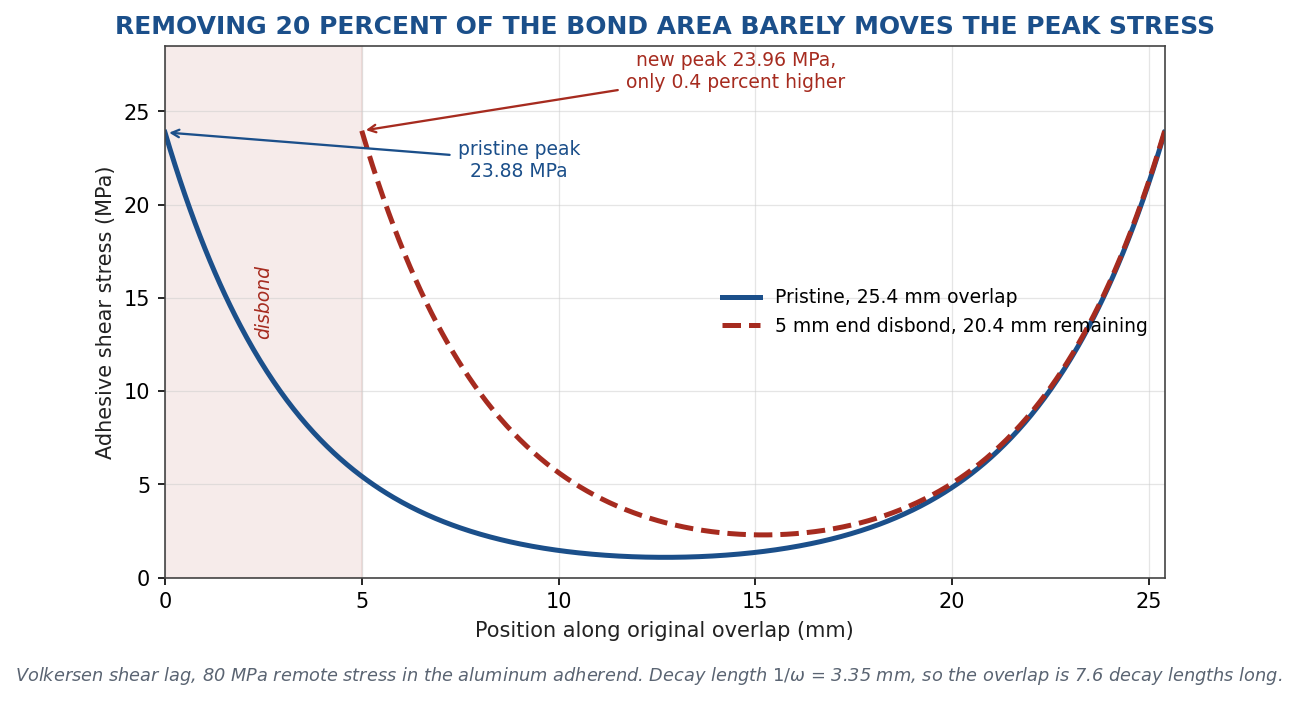
Figure 1. The disbond removes a fifth of the bond area and raises the peak adhesive shear stress by four tenths of one percent.
The peak goes from 23.88 MPa to 23.96 MPa. That is an increase of 0.4 percent. Push the disbond out to 10 mm, which is 39 percent of the bond area, and the peak rises by only 1.9 percent.
This is not a quirk of the numbers. It is what a long lap joint does. Once the overlap exceeds roughly four decay lengths, the peak adhesive stress becomes almost independent of overlap length, because the load transfer is controlled by the shear-lag decay and not by how much adhesive is present. Adding overlap to a long joint buys damage tolerance and inspection margin. It does not buy static strength.
So the residual static strength test is not failing to detect the damage. It is correctly reporting that the damage did not change the quantity it measures. A joint that lost 20 percent of its bond area will pass a static pull to within a few percent of pristine, which is well inside normal specimen scatter. The test is honest. It is just answering a different question than the one we care about.
Strength Is Linear. Life Is a Power Law.
Suppose an impact does elevate the local driving stress at the critical location, by a factor $k$, through resin microcracking, local fiber breakage, or load redistribution around a soft spot. Residual static strength scales roughly as $1/k$: you fail when the local stress reaches the local strength, so a 10 percent stress rise costs about 10 percent of strength.
Fatigue life does not behave that way. With a Basquin-type relation $N_f \propto \sigma^{-b}$, the life ratio is $k^{-b}$.
| Local stress rise | Static strength retained | Life retained, b = 3 | Life retained, b = 6 | Life retained, b = 10 |
|---|---|---|---|---|
| 5 percent | 95 percent | 86 percent | 75 percent | 61 percent |
| 10 percent | 91 percent | 75 percent | 56 percent | 39 percent |
| 20 percent | 83 percent | 58 percent | 34 percent | 16 percent |
| 35 percent | 74 percent | 41 percent | 17 percent | 5.0 percent |
| 50 percent | 67 percent | 30 percent | 8.8 percent | 1.7 percent |
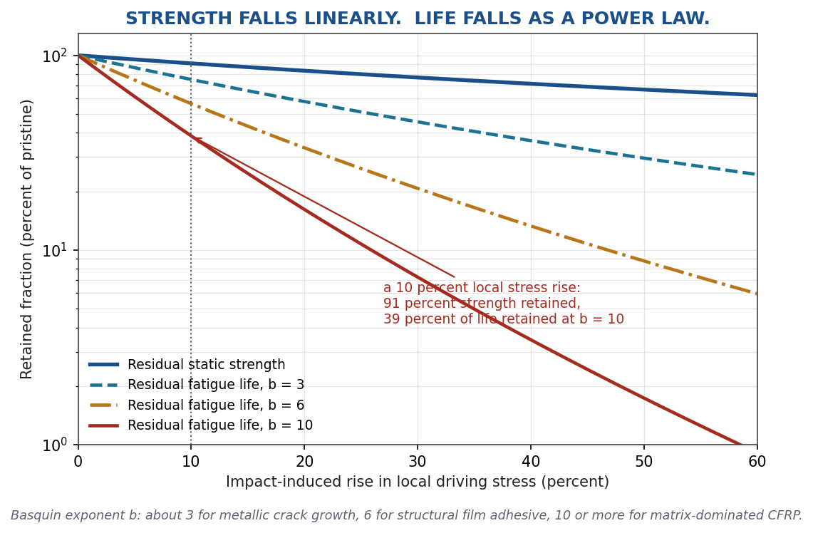
Figure 2. The gap between the two curves is the exponent. It is why a passing strength test is not reassurance.
A 10 percent local stress rise is invisible in a strength test. Specimen-to-specimen scatter in bonded joint strength is routinely larger than that. Yet at b = 10 it has taken 61 percent of the fatigue life.
The Flat S-N Curve Is Not the Good News It Sounds Like
Carbon composites are often praised for having flat S-N curves. The usual summary is that composites do not really fatigue the way metals do.
That summary hides a trap. A flat S-N curve means a large $b$. A large $b$ means life is hypersensitive to any change in stress. The same flatness that makes the material look forgiving in a constant-amplitude coupon test makes it unforgiving of a local stress elevation.
For unidirectional carbon in tension, $b$ can be 20 to 40. For quasi-isotropic laminates and for the matrix-dominated and bondline-dominated failure modes that actually govern a bonded joint, $b$ is more typically 6 to 12. Even at the low end of that range, the exponent is doing more damage to the life estimate than the strength loss suggests.
Metals are the opposite. A steep S-N curve, small $b$, means the material trades strength for life gradually. That is why intuition built on aluminum structure travels badly into composite structure.
What the Impact Actually Supplied
The power-law argument above is the conventional framing, and it is useful, but it still treats the problem as though we were sliding down a single S-N curve. For a bonded joint that framing is too generous.
A pristine bondline has no crack. Before a disbond can grow, one has to nucleate: the adhesive has to accumulate local damage at the overlap end until a separation forms. In most well-made bonded joints that nucleation phase is 60 to 90 percent of the total fatigue life. The joint spends most of its life not yet cracked.
Barely visible impact damage deletes that phase. The impact does not weaken the joint so much as it fast-forwards it. A structure that would have spent 80 percent of its life nucleating a disbond is handed one, pre-made, at exactly the overlap end where the peel and shear stresses peak.
That is why “how much life was lost” is the wrong question. What was lost was not a percentage. It was a phase.
A Threshold, Not a Knockdown Factor
Once a disbond front exists, the governing quantity is the strain energy release rate. For a long lap joint, the disbond reaches a steady state in which the energy released per unit of crack advance is independent of crack length: ahead of the front, the two adherends share load in parallel; behind it, one adherend carries everything. The difference is
$$G_{ss}=\frac{N^2}{2}\left[\frac{1}{E_1 t_1}-\frac{1}{E_1 t_1+E_2 t_2}\right]$$
where $N$ is the load per unit width. At 80 MPa remote stress this gives 37.8 J/m2.
Compare that against thresholds. A toughened epoxy film adhesive might have a mode II fatigue threshold near 60 J/m2 and a mode I threshold near 25 J/m2. A single-lap joint is mode II dominated. So the pristine design sits below its governing threshold with a margin of 1.59, and no disbond growth occurs at all. The joint is a runout.
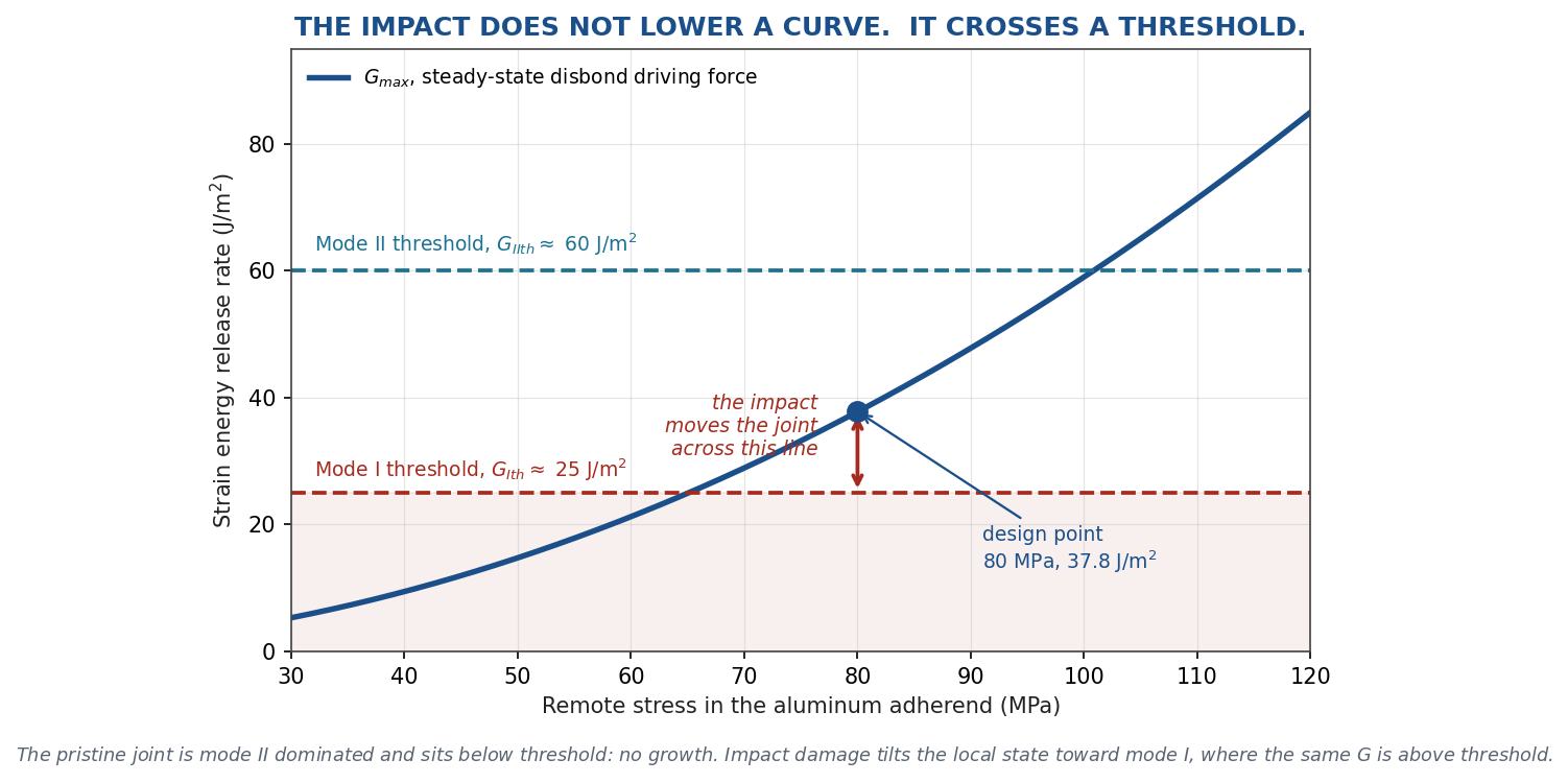
Figure 3. The impact does not move the design point. It moves the threshold that applies to it.
Impact damage changes the mode mix. A dent introduces local out-of-plane curvature; the adherend is no longer flat through the overlap end; the disbond front is no longer a clean mode II shear crack but a mixed-mode one with a peel component that was not there before. The applicable threshold drops toward the mode I value.
At 25 J/m2, the same 37.8 J/m2 design point is now above threshold by a factor of 1.51. Nothing about the load changed. Nothing about the bond area changed enough to matter. The joint simply moved from the no-growth regime into the growth regime.
This is the part that a knockdown factor cannot represent. The impact did not shave a curve downward by some percentage. It moved the joint across a threshold, from infinite life to finite life. That is a discontinuity, and no amount of multiplying the pristine S-N allowable by 0.8 will capture it.
How Long Is Ten Million Cycles?
Now the growth calculation. Using a Paris-type law in energy terms,
$$\frac{da}{dN}=C\left(\Delta G\right)^n$$
with $n$ = 5 and a rate anchored at one micrometer per cycle at 150 J/m2, the driving force of 37.8 J/m2 gives a growth rate of 1.0 nanometer per cycle. Growing the disbond from 5 mm to 15 mm therefore takes 9.9 million cycles.
Nine point nine million cycles sounds like a comfortable number. Whether it is depends entirely on how fast the structure accumulates cycles, and that is a question about the frequency content of the service environment rather than about the damage.
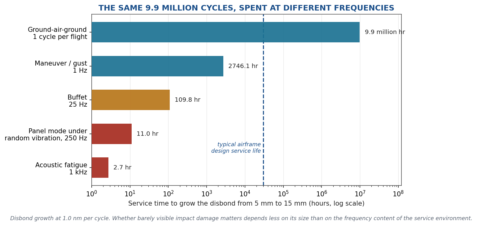
Figure 4. The same crack, the same growth rate, and five completely different verdicts.
On a ground-air-ground cycle, one per flight, 9.9 million cycles will never be reached in any service life. The damage is genuinely benign and the airplane will be retired long before the disbond notices. On a 1 Hz maneuver and gust spectrum it is 2,700 hours, which is a real inspection problem but a manageable one.
At 25 Hz, in buffet, it is 110 hours. At a 250 Hz panel mode under random vibration it is 11 hours. Under acoustic excitation at 1 kHz it is under three hours.
An engineer looking at that disbond in an airframe fuselage panel and an engineer looking at the identical disbond in a launch vehicle payload fairing or an engine nacelle acoustic liner are looking at two different problems. The first has a maintenance item. The second has a structure that may not survive a single qualification test, let alone a mission.
The Modal Survey Will Mislead You
A natural instinct is to run a modal survey before and after impact and watch for a frequency shift. This deserves a warning.
The frequency shift from local stiffness loss is weighted by the fraction of the mode’s strain energy in the damaged region:
$$\frac{\Delta f_r}{f_r}\approx-\frac{1}{2}\gamma_r\frac{\Delta k}{k}$$
For a BVID zone occupying 2 percent of the mode’s strain energy region with a 40 percent local stiffness loss, the shift is 0.4 percent. Composite structures routinely move more than that with temperature and moisture. The damage indicator is smaller than the environmental noise floor.
Worse, the modal metrics can move in the reassuring direction. Delamination and disbond faces rub, and that friction adds damping. Take a bonded panel with a 250 Hz mode at Q = 25 under a 0.04 G2/Hz input. Miles gives
$$G_{RMS}=\sqrt{\frac{\pi}{2}f_n Q P}$$
which is 19.8 GRMS. After impact, with the frequency down 0.5 percent and the loss factor up 40 percent, the response falls to 16.7 GRMS. That is a 16 percent reduction in response. Run that through a conventional S-N bookkeeping at b = 10 and the apparent damage rate drops to 18 percent of the pristine value.
So the impacted panel reports a lower vibration response and a lower calculated fatigue damage rate than the pristine one, while a disbond grows underneath it at a nanometer per cycle. The added damping is a symptom of the damage, and treating it as an improvement in the environment is exactly backwards.
I have written before about the same trap in bridge structural health monitoring, where a restrained bearing raises a frequency and midspan stiffness loss lowers it, so two opposing defects can hold the measured frequency perfectly stable. The composite version is worse, because here the two effects both come from the same defect.
The deeper reason the S-N bookkeeping goes wrong is that it is the wrong bookkeeping. Rainflow and Miner are counting a nucleation process that already finished. Once a crack front exists, the relevant integral is over crack growth, and crack growth responds to the largest cycles and to the mode mix rather than to the RMS. This is the same distinction I have raised regarding peak distributions in random vibration: the effect on rainflow damage and the effect on crack growth are not the same, and crack growth is the more sensitive of the two.
What About Stiffness Degradation?
Everything above has treated the damage through strength and through fracture mechanics. There is a third framework, and in composite fatigue work it is often the preferred one: track the stiffness.
The reasoning behind it is sound. Miner’s rule struggles in composites because there is no single dominant crack and no clean cycle-counting analogue for distributed matrix damage. Stiffness, by contrast, is a directly measurable state variable that declines monotonically as damage accumulates. So instead of counting cycles, you track the normalized modulus and treat it as the damage variable.
A composite laminate under cyclic load loses stiffness in three recognizable stages. Stage I is a rapid initial drop as transverse matrix cracks form and multiply until they reach a saturation spacing, typically costing a few percent of modulus within the first ten percent of life. Stage II is a long, slow, quasi-linear decline as delaminations initiate at crack tips and free edges. Stage III is a runaway drop in the final few percent of life as fiber-dominated failure takes over.
The tempting move is obvious. Measure residual stiffness after the impact, find that value on the pristine degradation curve, and read off how much life the impact consumed. It is non-destructive, it is cheap, and unlike residual strength it actually responds to the damage.
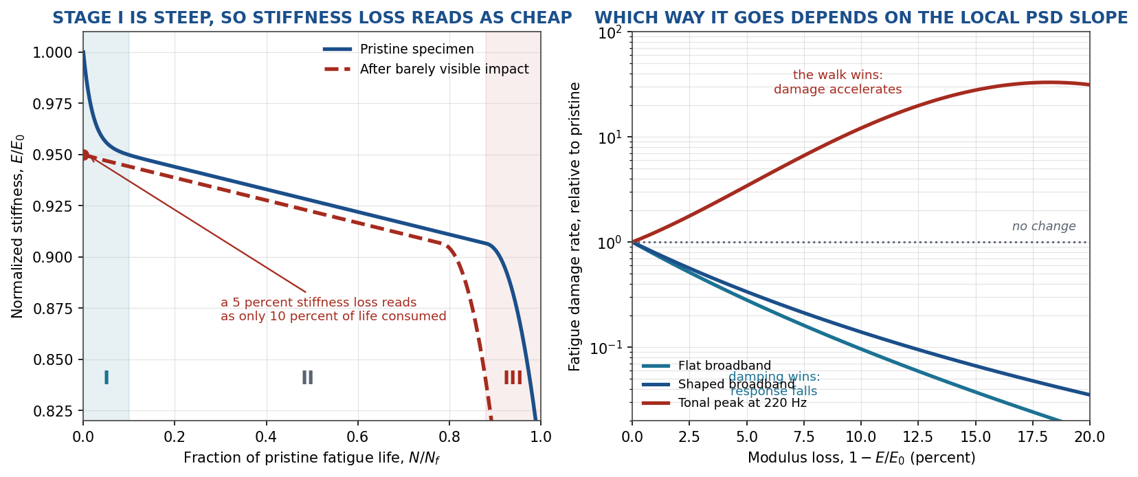
Figure 5. Left: the impacted specimen enters the pristine curve at ten percent of life. Right: whether progressive degradation raises or lowers the calculated damage rate depends entirely on the local slope of the input spectrum.
It does not work, and the left panel of Figure 5 shows why. Because Stage I is steep, a 5 percent stiffness loss lands at a normalized life of only 0.10. The stiffness bookkeeping reports that the impact consumed ten percent of the fatigue life.
Set that against the earlier fracture mechanics result, where the same damage moved the joint from below its disbond threshold to above it, converting a runout into a finite life. Ten percent is not a small error. It is the wrong answer.
The failure is in the mapping, not in the measurement. Reading a stiffness loss off the pristine curve assumes the damage that produced it is the same kind of damage the curve was built from. Stage I stiffness loss comes from distributed matrix cracking that saturates and then largely stops, and it is genuinely benign: a lot of small cracks, no dominant one, no stress concentration. Barely visible impact damage produces a comparable global stiffness signature from a completely different local state, namely a crack front sitting at the peak-stress location. Equal stiffness does not mean equal damage.
So residual stiffness joins residual strength on the list of measurements that are honest about what they measure and misleading about what we want to know. Both are volume-averaged quantities. Impact damage is a local event. Averaging is exactly the operation that destroys the information.
Where Stiffness Degradation Does Matter
Having argued that stiffness is a poor damage metric here, I want to argue that it is an important quantity for a different reason. It moves the natural frequency, and the natural frequency sets the vibration environment.
This appears to contradict the earlier modal section, where the frequency shift from impact damage was only 0.4 percent and was buried inside temperature and moisture drift. The two results are consistent, and the distinction is worth stating plainly.
The frequency shift is weighted by the fraction of the mode’s strain energy in the damaged region. For a localized dent, that fraction is a couple of percent, so the shift is negligible. For progressive stiffness degradation distributed across the whole panel, the fraction approaches unity and the shift follows the modulus directly:
$$\frac{f_n}{f_{n0}}=\sqrt{\frac{E}{E_0}}$$
A 10 percent modulus loss moves a 250 Hz panel mode to 237 Hz. That is not a subtle shift, and it is easily measurable. Frequency tracking is a poor detector of localized impact damage and a good tracker of global progressive degradation. Those are different jobs, and conflating them is how monitoring programs end up disappointed.
Now the consequence. As the panel degrades, two things happen at once and they push in opposite directions. The frequency falls, which walks the mode to a new point on the input spectrum. The loss factor rises, because delamination and matrix crack faces rub. Miles gives the response as the product of the three, so
$$G_{RMS}\propto\sqrt{f_n\,Q\,P(f_n)}$$
and the question of whether the damage rate climbs or falls is settled by the local slope of the PSD.
| Modulus retained | Mode frequency | Loss factor | Damage rate, broadband | Damage rate, tonal |
|---|---|---|---|---|
| 100 percent | 250.0 Hz | 1.00 | 1.00 | 1.0 |
| 95 percent | 243.7 Hz | 1.25 | 0.33 | 3.5 |
| 90 percent | 237.2 Hz | 1.50 | 0.14 | 11.7 |
| 85 percent | 230.5 Hz | 1.75 | 0.067 | 27.6 |
| 80 percent | 223.6 Hz | 2.00 | 0.035 | 31.3 |
For a flat or gently shaped broadband input, the damping rise wins comfortably. At 20 percent modulus loss the calculated damage rate has fallen to a few percent of pristine. This is the same trap as before, arriving from a new direction: a panel that is visibly degrading reports a falling fatigue damage rate.
For a tonal or narrowband environment the verdict reverses. If the mode walks toward a spectral peak rather than away from one, the rise in input outruns the damping and the damage rate climbs by a factor of thirty. Nothing about the excitation changed. The structure simply moved into it.
The break-even condition is worth carrying around. The walk overcomes the damping when
$$\frac{P(f_n)}{P(f_{n0})}>\frac{\eta/\eta_0}{\sqrt{E/E_0}}$$
For the numbers above at 20 percent modulus loss, the input has to rise by 124 percent across the frequency walk, which corresponds to the mode sitting on a spectral skirt steeper than roughly 43 dB per octave. Broadband qualification spectra are rarely that steep. The skirts of engine orders, blade passing tones, and lightly damped upstream resonances routinely are.
The Bondline Version of the Same Trap
The adhesive layer degrades too, and it produces the most counterintuitive result in this post.
Return to the shear-lag parameter from the demonstration joint. The adhesive modulus appears in the numerator, so softening the bondline reduces $\omega$ and lengthens the load-transfer decay length. A longer decay length spreads the load transfer over more of the overlap, which lowers the peak.
| Adhesive shear modulus | Decay length 1/ω | Peak adhesive shear | Change |
|---|---|---|---|
| Pristine, 1.10 GPa | 3.35 mm | 23.88 MPa | — |
| 0.83 GPa, 25 percent softer | 3.87 mm | 20.72 MPa | −13.2 percent |
| 0.66 GPa, 40 percent softer | 4.33 mm | 18.58 MPa | −22.2 percent |
| 0.55 GPa, 50 percent softer | 4.74 mm | 17.03 MPa | −28.7 percent |
A bondline that has lost half its shear modulus carries a peak shear stress 29 percent lower than the pristine one. Adhesive softening is self-relieving in a lap joint. Any check based on peak adhesive stress will report improvement.
The improvement is real, in the narrow sense that the peak stress genuinely is lower. It is also irrelevant, because the adhesive’s strength and its threshold have degraded alongside its modulus, and the ratio that actually matters has gone the wrong way.
On the NDI Question
The original post asked which inspection methods reliably catch barely visible impact damage. The honest answer is that the choice depends on which failure mode you are worried about, and that one method in particular is worth more attention than it usually gets.
| Method | Delamination in the laminate | Disbond in the adhesive | Kissing bond |
|---|---|---|---|
| Visual, tap test | Poor | Gross disbonds only | No |
| Phased array UT, C-scan | Excellent, maps depth | Good if an air gap exists | No |
| Flash and pulsed thermography | Good to a few mm depth | Good, fast over large area | No |
| Vibrothermography | Good | Good | Yes, heats by friction |
| Shearography | Fair | Good, full field, needs load | Poor |
| X-ray computed tomography | Excellent | Fair, thin bondline | No |
| Acoustic emission under proof load | Detects active growth | Detects active growth | Yes if it moves |
| Frequency and mode shape tracking | Poor for small BVID | Poor | No |
| Modal loss factor | Good | Good | Fair |
| Nonlinear acoustics, vibro-acoustic modulation | Excellent | Excellent | Yes |
The kissing bond column is the one that matters most for adhesive joints, and it is the column where conventional ultrasonics fails. A kissing bond is a disbond whose faces remain in intimate contact. There is no air gap, so there is almost no acoustic impedance mismatch, so a pulse-echo inspection sees a bonded interface. The joint can be nearly zero-strength in peel and look perfect on a C-scan.
Why Nonlinear Methods Win Here
Vibro-acoustic modulation exploits the fact that a closed crack is a nonlinear element. Drive the structure with a low-frequency pump tone at a convenient structural mode, which alternately opens and closes the crack faces. Simultaneously inject a high-frequency ultrasonic probe tone. In an undamaged structure the two pass through independently. In a damaged one the crack modulates the probe wave, and sidebands appear at the probe frequency plus and minus the pump frequency.
The modulation index, the sideband amplitude ratioed to the carrier, is the damage indicator. A pristine joint sits at the instrumentation and material nonlinearity floor, typically below 0.001. Impact damage pushes it to 0.01 or higher.
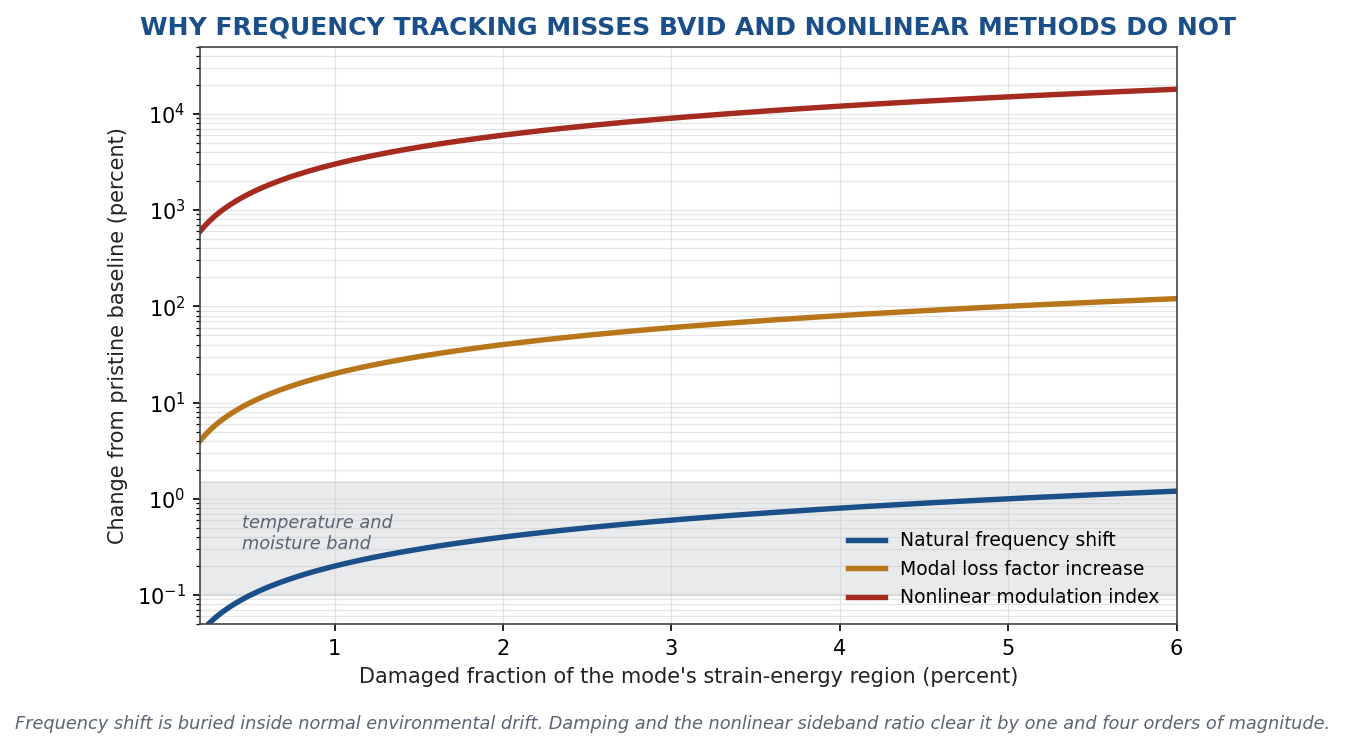
Figure 6. Four decades separate the least sensitive damage indicator from the most sensitive one.
The sensitivity ladder is stark. At 2 percent damage extent the frequency has moved 0.4 percent, which is inside the environmental band. The loss factor has moved 40 percent, which is detectable but requires a good baseline. The modulation index has moved by a factor of sixty.
There is a second advantage that gets less attention than it deserves. Linear frequency-shift monitoring requires a pristine baseline and requires that baseline to be corrected for temperature, moisture, and boundary condition drift. Nonlinear modulation is closer to a zero-baseline method: a linear structure produces no sidebands, so the absence of sidebands is itself the healthy condition. You are not comparing against a remembered number that may have drifted.
What I Would Do Instead
Four recommendations follow from the above.
Stop treating residual static strength as the acceptance criterion. Compression after impact per ASTM D7137 is a useful material screening test and a poor structural clearance test. It measures the quantity least affected by the damage. Residual stiffness is no better, for the reasons in Figure 5: it responds to the damage but maps it onto the wrong curve. If a fatigue-after-impact test is affordable, run that instead. If it is not, at least run the damage tolerance analysis.
Treat the impact site as an initial flaw and do the fracture mechanics. The size of that flaw is not the size of the visible dent. It is the largest flaw the chosen inspection method could plausibly miss. That closes the loop between the NDI selection and the analysis, in the same way that detectable crack size drives inspection intervals in metallic damage tolerance.
Design the bondline so that the steady-state release rate stays below threshold even with that flaw present, and check the threshold in mode I, not mode II. In the example joint, the mode II threshold permits 101 MPa and the mode I threshold permits only 65 MPa. Designing to the mode II number and then discovering the mode I number after an impact is the failure mode this whole post is about. If the joint is below the mode I threshold at limit load, disbond growth cannot initiate regardless of what the impact did, and the problem becomes self-limiting.
Match the inspection interval to the frequency content, not to the calendar. Figure 4 is the argument. The same disbond is a thirty-year problem in one environment and a one-afternoon problem in another. An inspection program written in flight hours for a structure whose governing environment is a 250 Hz panel mode is measuring the wrong clock.
Closing
The original post described a structure that passes its strength test and is counting down to fatigue failure. That framing is right, and I would sharpen it in one respect.
The countdown did not start because the impact removed strength. It started because the impact removed the nucleation phase and shifted the mode mix at the overlap end, moving a joint that was sitting comfortably below its disbond threshold to a joint sitting above it. The static test could not see any of that, because none of it is a strength quantity.
The uncomfortable part is that every one of the usual reassurances points the wrong way. The strength test passes. The frequency survey shows no meaningful shift. The residual stiffness maps onto the pristine curve at ten percent of life consumed. The vibration response goes down, because the damage added damping. And in the bondline, softening the adhesive lowers the peak shear stress. Five independent measurements, all saying the structure is fine, every one of them technically correct, and a disbond growing the whole time.
The methods that see through this are the ones sensitive to the existence of an interface rather than to the amount of material: nonlinear acoustics, vibrothermography, acoustic emission under load. Those are the ones I would put my money on.
Related reading on this site: Nastran SOL 111 versus SOL 112 for rainflow and crack growth, which develops the distinction between spectral damage bookkeeping and cycle-by-cycle crack growth that appears above.
My free ebooks, including one on composite fatigue, are available at Tom’s Ebooks.
The demonstration joint and its properties are generic and are used only to keep the comparisons on a common basis. They do not represent any specific program hardware. Threshold and growth-rate values are representative of structural film adhesives and should be replaced with qualification data for any real assessment.