SOL 111 or SOL 112? Why a Synthesized Time History Earns Its Keep
A base input power spectral density arrives on a specification sheet, and the reflex is automatic. Build the model, run SOL 111, read the RMS stress, apply a three-sigma factor, and compare against allowable. The whole exercise takes an afternoon on a model of any reasonable size, and for a great many components that is exactly the right level of effort.
But the moment somebody downstream asks for a rainflow cycle count, a NASGRO crack growth spectrum, a shock response spectrum of the response, or an answer that includes a gap or a snubber or a friction interface, the frequency domain quietly stops being able to help. The information those tasks need was thrown away at the first step, when the phase was discarded.
This article works a small example both ways. The frequency domain answer and the time domain answer agree on the one number they can both produce. Then the time domain keeps going.
The Demonstration Model
Consider a bracket carrying an electronics box, mounted to a structure that shakes in one direction. The stress of interest is at a fillet radius. Three elastic modes participate: 78, 190 and 460 Hz, each with an amplification factor $Q=10$, which is 5 percent of critical damping. Each mode contributes stress at the fillet in proportion to the base acceleration, with quasi-static coefficients of 600, 280 and 170 psi per G respectively.
The base input is the flat-topped random vibration specification in Figure 1, running from 20 to 2000 Hz at an overall level of 4.57 GRMS. The first two modes sit squarely on the plateau. The third sits on the roll-off.
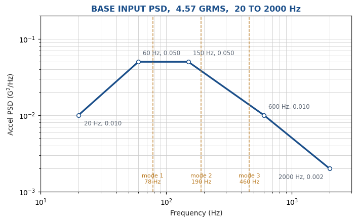
Figure 1. The base input specification. The three participating modes are marked in amber.
What SOL 111 Actually Computes
SOL 111 is modal frequency response with a random analysis module bolted on the end. Nastran first solves the deterministic frequency response problem for a unit input, producing a complex transfer function $H(f)$ between the input and every requested output item. The RANDPS entry then names the input PSD, given as a TABRND1 table, and the random module forms the output PSD one frequency line at a time:
$$S_{xx}(f)=\left|H(f)\right|^{2}S_{ff}(f)$$
Note what happened to the phase. It was squared away. What comes out is a real, non-negative function of frequency, and the statistics that can be recovered from it are exactly the spectral moments:
$$m_n=\int_{0}^{\infty}f^{\,n}\,S_{xx}(f)\,df$$
The RMS is $\sigma=\sqrt{m_0}$. The zero up-crossing rate is $\nu_0=\sqrt{m_2/m_0}$, the peak rate is $\nu_p=\sqrt{m_4/m_2}$, and the irregularity factor is $\gamma=\nu_0/\nu_p$. That is the complete inventory. Everything a spectral fatigue method can ever tell you is built from those moments.
For the demonstration model, integrating the response PSD gives a fillet stress of 5751 psi RMS, with $\nu_0=171.0$ up-crossings per second, $\nu_p=395.6$ peaks per second, and $\gamma=0.432$. That last number is the tell. An irregularity factor of 0.43 is a long way from unity, which means the response is genuinely broadband and there are more than two peaks for every mean-level crossing.
It is worth pausing on the Miles equation here, because it is the check almost everyone runs first:
$$\sigma_a=\sqrt{\frac{\pi}{2}\,f_n\,Q\,A(f_n)}$$
Applied to the fundamental mode alone, Miles returns 4696 psi RMS against the full three-mode answer of 5751 psi. It is 18 percent low, because the second and third modes together carry a third of the mean square. Miles is a single-degree-of-freedom formula and it should be treated as a sanity check, not as an analysis.
Why Either Domain Works, and Where That Stops
It is worth being precise about why a time domain solution and a frequency domain solution are entitled to agree, because the same argument shows exactly where they part company.
Start with the Fourier transform pair:
$$X(f)=\int_{-\infty}^{\infty}x(t)\,e^{-i2\pi ft}\,dt\qquad\qquad x(t)=\int_{-\infty}^{\infty}X(f)\,e^{i2\pi ft}\,df$$
The transform is invertible. Nothing is lost going either way, because $X(f)$ is complex and carries both magnitude and phase. A time history and its Fourier transform are two representations of the same object, and any question that can be answered from one can be answered from the other.
Plancherel’s theorem makes the bookkeeping exact. The Fourier transform is a unitary operator on the square-integrable functions, so it preserves inner products. The special case of a function taken with itself is Parseval’s theorem:
$$\int_{-\infty}^{\infty}\left|x(t)\right|^{2}dt=\int_{-\infty}^{\infty}\left|X(f)\right|^{2}df$$
A stationary random process is not square-integrable. It has finite power rather than finite energy, so the statement has to be made per unit time, and what it returns is the mean square:
$$\lim_{T\to\infty}\frac{1}{T}\int_{0}^{T}x^{2}(t)\,dt=\int_{0}^{\infty}S_{xx}(f)\,df=m_0=\sigma^{2}$$
This is why the SOL 111 RMS and the SOL 112 RMS have to match. The agreement is not evidence that the model is good, and it is not a lucky coincidence. It is Parseval’s theorem. If the two numbers disagree by more than the numerical tolerances, one of the two decks is wrong.
The Wiener-Khinchin theorem then says what a PSD actually is. It is the Fourier transform of the autocorrelation function:
$$S_{xx}(f)=\int_{-\infty}^{\infty}R_{xx}(\tau)\,e^{-i2\pi f\tau}\,d\tau\qquad\qquad R_{xx}(0)=\sigma^{2}$$
Read that carefully. The PSD is equivalent to the autocorrelation, which is a second-order statistic. It is not equivalent to the signal.
Laplace covers the structural half of the problem. In the time domain the response is the convolution of the input with the impulse response, which is Duhamel’s integral:
$$y(t)=\int_{0}^{t}h(t-\tau)\,x(\tau)\,d\tau$$
Transform it and convolution becomes multiplication, $Y(s)=H(s)X(s)$, where for a viscously damped single-degree-of-freedom oscillator
$$H(s)=\frac{1}{s^{2}+2\zeta\omega_n s+\omega_n^{2}}$$
The frequency response function that SOL 111 builds is this same transfer function evaluated on the imaginary axis, $s=i2\pi f$. There is one operator here, viewed from two sides. SOL 112 evaluates it by marching the convolution forward in time. SOL 111 evaluates it by multiplying at each frequency line. Provided the system is linear and stable, with all poles in the left half of the s plane, and provided the startup transient has decayed, the two must give the same steady-state answer.
So far the two domains are interchangeable. The break comes at one specific step, the same step flagged earlier:
$$S_{xx}(f)=\lim_{T\to\infty}\frac{1}{T}\,E\!\left[\left|X_T(f)\right|^{2}\right]$$
Here $X_T(f)$ is the transform of one finite-length record and $E$ denotes the expected value. Squaring a magnitude is not invertible. The Fourier transform carries one time history to one spectrum and back again, but the PSD carries an infinite family of time histories onto a single curve. Every member of that family has the same RMS, the same spectral moments and the same crossing rates. They do not have the same peaks, the same cycle sequence or the same rainflow content. Synthesis is the act of picking one member of that family by assigning phase.
Figure 2 makes the point with three stress records built from the same PSD using three different sets of random phase.
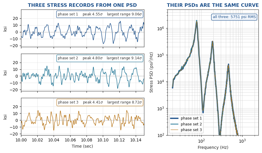
Figure 2. One PSD, three phase sets, three different records. The RMS is identical. The peaks are not.
All three have an RMS of 5751 psi, identical to within round-off, exactly as Parseval requires. Their largest peaks are $4.55\sigma$, $4.80\sigma$ and $4.41\sigma$, and their largest rainflow ranges are $9.06\sigma$, $9.14\sigma$ and $8.72\sigma$. Across five phase sets the total fatigue damage varied by only 0.8 percent at $b=3$ and 4.2 percent at $b=6.4$, while the largest peak varied by 9 percent. Cumulative quantities that average over tens of thousands of cycles are very nearly fixed by the PSD. Extreme values are not, and neither is anything that depends on the order in which the cycles arrive.
Two further assumptions hide inside the equivalence, and both bite in practice. The first is superposition. A nonlinear system has no transfer function at all, because $H(s)$ is defined only for a linear operator. That is the mathematical reason SOL 111 cannot represent a gap, rather than merely a software limitation. The second is stationarity. Wiener-Khinchin presumes the autocorrelation depends on the lag alone and not on absolute time. A mission profile whose level changes is not stationary, and one PSD computed across the whole record describes no part of it.
Synthesizing a Time History That Matches the PSD
The alternative path starts by manufacturing an acceleration time history whose power spectral density matches the specification. The classical approach is the one described by David Smallwood: assign the target magnitude to each spectral line, assign an independent uniformly distributed random phase to each line, take the inverse FFT, and then iterate the magnitudes a handful of times so that the realized PSD converges onto the target.
The synthesis here produced 120 seconds at 20,480 samples per second, which is 2,457,600 points. The realized time history has an overall level of 4.571 GRMS against the specification value of 4.571 GRMS, a kurtosis of 3.00, and a crest factor of 5.38. Those three checks matter. A synthesized record that misses the RMS is useless, a record with kurtosis far from 3.0 is not the Gaussian process the specification implies, and a record whose crest factor is stuck near 3.0 has been clipped somewhere in the generation chain.
Two more decisions matter as much as the synthesis itself. The sample rate has to be high enough that the highest frequency of interest is resolved rather than merely captured, which in practice means at least ten points per cycle at the top of the band, not the two that Nyquist permits. And the duration has to be long enough that the largest cycles are represented. A 5 second record does not contain the rare high peaks that a 10 minute exposure will produce, and fatigue and crack growth both live in that tail.
The SOL 112 Run
SOL 112 is modal transient response. The base motion is normally applied by the large mass method: a very large mass on a CONM2 at the drive point, a SUPORT on the driven degree of freedom, and a force applied through DAREA and TLOAD1 equal to the large mass times the desired acceleration. The synthesized acceleration goes into the deck as a TABLED1 or TABLED2 referenced by the TLOAD1, and TSTEP sets the integration step and the output interval.
Figure 3 shows a 0.15 second window of the synthesized base input and the resulting fillet stress. The character of the two records is different in a way that no PSD plot conveys. The input looks like broadband noise. The stress carries a visible 78 Hz rhythm with the higher modes riding on it, and a scatter of small excursions between the large ones.
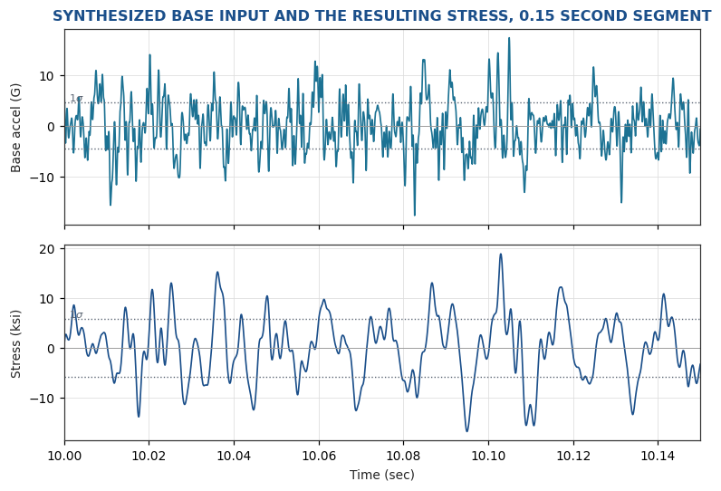
Figure 3. A short segment of the synthesized base input and the SOL 112 fillet stress. The dotted lines are the one-sigma levels.
Nastran does not stop when a TABLED entry runs out of data. It extrapolates linearly from the last two points, silently, for as long as TSTEP asks it to. If the TSTEP duration exceeds the length of the input table, the solution will ramp away from the physics and the response will be nonsense that still looks like a converged answer. Check that the last time value in the table is at least as large as the number of steps times the step size, on every run, every time.
The Cross-Check
Before the time domain result can be used for anything, it has to reproduce the frequency domain result. Figure 4 overlays the SOL 111 stress PSD on the PSD computed from the SOL 112 stress time history. They lie on top of one another, including the anti-resonance notches between modes.
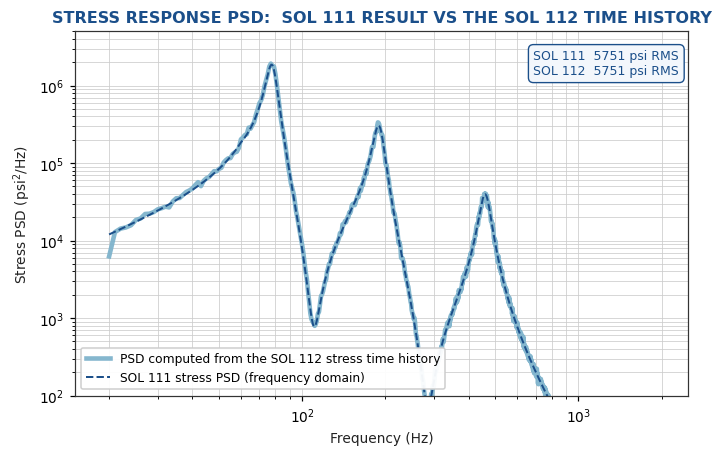
Figure 4. The frequency domain and time domain stress PSDs agree line for line.
The agreement in this idealized example is essentially exact, because the synthesized input matches the specification line by line and both solutions use the same modal basis. On a real model with tens of thousands of elements, expect and demand agreement within about one percent. Anything worse points at a real defect: modal truncation, a residual vector request that is present in one deck and missing from the other, a damping table that was translated incorrectly, or a frequency grid too coarse to resolve a lightly damped peak. That one-percent check is the single most valuable thing about running both solutions, and it costs almost nothing once the decks exist.
| Quantity | SOL 111 | SOL 112 |
|---|---|---|
| Fillet stress, RMS (psi) | 5751 | 5751 |
| Zero up-crossings per second | 171.0 | 171.1 |
| Peaks per second | 395.6 | 395.3 |
| Irregularity factor | 0.432 | 0.433 |
| Largest absolute peak | not available | 27,681 psi |
| Rainflow cycles in 120 sec | not available | 47,432 |
| Cycle mean stress distribution | not available | 3916 psi std dev |
Table 1. What each solution delivers for the same problem.
The Peaks Are Not Rayleigh
A stubbornly common belief holds that the absolute peaks of a stationary Gaussian random response follow the Rayleigh distribution. That is true only in the narrowband limit, where the irregularity factor approaches unity. This response has $\gamma=0.433$, and Figure 5 shows what that does.
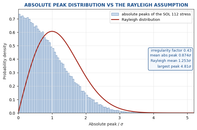
Figure 5. The absolute peaks pile up near zero and also reach further than Rayleigh allows.
The mean absolute peak is $0.874\sigma$ against the Rayleigh value of $1.2533\sigma$. Nearly 35 percent of the peaks fall below half a sigma, where the Rayleigh distribution predicts 12 percent. Those small peaks are the little wiggles of the higher modes riding on the fundamental, and they contribute essentially nothing to fatigue. At the other end, the largest peak in the 120 second record reached $4.81\sigma$.
The peak stress in this record is 1.60 times the three-sigma value. Three sigma is not a peak. It is a level exceeded on roughly 0.27 percent of samples, and this record contains 480 individual peaks above it. For a peak estimate, use $\sqrt{2\ln(\nu_0 T)}$, which gives $4.46\sigma$ here, or simply read the peak off the time history that SOL 112 already produced.
Rainflow Cycle Counting
Rainflow counting per ASTM E1049 needs a sequence of turning points. It cannot be performed on a PSD. The SOL 112 stress record yielded 94,864 turning points and 47,432 rainflow cycles over 120 seconds. Figure 6 compares the resulting range histogram with the narrowband prediction.
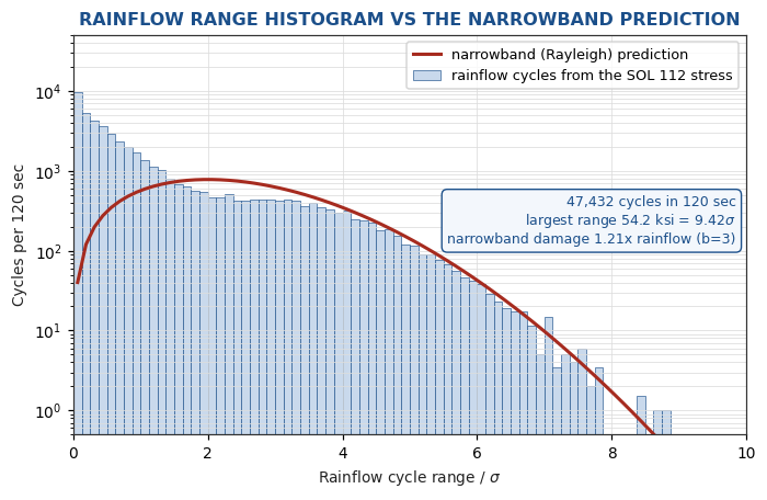
Figure 6. Rainflow range histogram against the narrowband prediction. Note the log scale on the count axis.
The narrowband model predicts $\nu_0 T=20{,}521$ cycles. The actual count is 47,432, more than twice as many, and the excess is almost entirely in small ranges. The narrowband model also falls below one cycle per record at a range of about $8.3\sigma$, while the record contains cycles out to $9.42\sigma$, a range of 54.2 ksi.
Now take those cycles into Miner’s rule with $N=A\,S_a^{-b}$ and compare the damage against the two standard spectral estimates. The narrowband closed form is
$$D_{nb}=\frac{\nu_0 T}{A}\left(\sqrt{2}\,\sigma\right)^{b}\Gamma\!\left(1+\frac{b}{2}\right)$$
and Dirlik’s method builds an amplitude density from one exponential and two Rayleigh terms, with coefficients derived from $m_0$, $m_1$, $m_2$ and $m_4$. For this response Dirlik returns $D_1=0.243$, $D_2=0.432$, $D_3=0.326$, $Q=0.303$ and $R=0.111$.
| Method | Damage ratio, $b=3$ | Damage ratio, $b=6.4$ |
|---|---|---|
| Rainflow of the SOL 112 record | 1.000 | 1.000 |
| Narrowband, from the SOL 111 PSD | 1.211 | 1.141 |
| Dirlik, from the SOL 111 PSD | 0.945 | 0.866 |
Table 2. Fatigue damage relative to the rainflow result, for two S-N exponents.
Two observations follow. The narrowband estimate is conservative, by 21 percent at $b=3$ and 14 percent at $b=6.4$, which for a screening calculation is perfectly acceptable. Dirlik is closer but lands on the unconservative side, by 6 percent at $b=3$ and 13 percent at $b=6.4$. That trend is worth flagging: as the S-N exponent rises, the estimate leans harder on the shape of the extreme tail, which is precisely where a three-term fitted density is least reliable. This is the motivation behind corrections such as Meta-Dirlik.
For total fatigue damage under a stationary Gaussian input, the spectral methods are good enough that the extra work of SOL 112 is hard to justify on damage alone. The case for the time history is built elsewhere.
NASGRO and Crack Growth
Damage tolerance analysis is where the frequency domain runs out of road entirely. Crack growth is an integration of $da/dN$ cycle by cycle, and the growth rate depends on the stress intensity range and on the stress ratio $R=S_{min}/S_{max}$. A PSD carries no information about $R$ at all. Every cycle it implies is fully reversed about zero.
The SOL 112 record tells a different story. The rainflow cycle means have a standard deviation of 3916 psi, which is $0.681\sigma$, with the 5th and 95th percentiles at roughly plus and minus 6.6 ksi. Individual cycles in a zero-mean random response are frequently offset well away from zero, because a small high-frequency cycle can sit near the crest of a large low-frequency one. That is a real mean stress on that cycle, and NASGRO will treat it as one.
There is a practical choice about what to hand the crack growth code. A pre-counted max/min/cycles spectrum file is compact and easy to review, but the counting has already been done and the sequence is gone. Handing over the turning point sequence instead lets NASGRO perform its own cycle counting and preserves the order in which the cycles occur. Sequence matters if retardation models are switched on, and it also matters for how the code assembles its load blocks. The tradeoff is file size and the risk of format mismatches. It is worth checking carefully how the receiving code interprets the columns of whatever file is delivered, because a misread that quietly multiplies the load can produce a life estimate that is wrong by orders of magnitude while looking entirely plausible.
A related judgment call is amplitude gating. Most of the 47,432 cycles are tiny and contribute almost no damage, but they dominate the file size. Gating at a threshold and reporting the damage fraction discarded is standard practice. For this record, discarding every rainflow cycle whose range is below half a sigma removes 48 percent of the cycles and 0.09 percent of the damage at $b=3$. Always compute and report the discarded fraction rather than assuming it.
Nonlinear Analysis
SOL 111 is linear by construction. The random module assumes superposition. A gap, a snubber, a bolted joint that slips, a rubber isolator that stiffens under strain, a fastener that goes into bearing, a cable that only takes tension, an amplitude-dependent damping law: none of these can be represented, and there is no correction factor that rescues the answer.
A quick numerical experiment makes the point. Take the fundamental mode of the demonstration model as a single-degree-of-freedom oscillator, driven by the same synthesized base input, and add a travel-limiting snubber that engages at 1.5 sigma of the linear relative displacement and quadruples the stiffness beyond that point. Direct integration of the nonlinear equation of motion gives:
| Relative displacement | Linear | With snubber | Change |
|---|---|---|---|
| RMS (inch) | 0.01231 | 0.00993 | 19 percent lower |
| Peak (inch) | 0.05290 | 0.03462 | 35 percent lower |
| Relative fatigue damage, $b=3$ | 1.000 | 0.655 | 35 percent lower |
Table 3. Effect of a travel-limiting snubber, which SOL 111 cannot represent at all.
The snubber cuts the peak displacement by 35 percent, which is the whole reason it is there. But it does so by transferring load into whatever the snubber bears against, and by pushing energy up in frequency into components that the linear model never sees. A linear analysis is conservative for the isolated mass and unconservative for the stop. Neither error is visible without a time domain solution.
Everything Else That Comes Free With a Time History
Once the response time history exists, a long list of downstream tasks becomes routine rather than impossible.
Shock response spectra. An SRS of the response acceleration is a direct calculation from a time history and is undefined from a PSD. If the random environment has to be compared against or combined with a shock environment, the time history is the common currency.
Combining with quasi-static loads. A buffet or acoustic response record contains no maneuver loads, no thrust, no thermal. Those have to be superimposed before the spectrum means anything for the real mission. Superposition on a time history is straightforward. Superposition on a PSD is not, and combining the two by root-sum-square discards exactly the mean stress information that crack growth depends on.
Non-Gaussian and non-stationary environments. Real flight and transport data are often kurtotic, and levels vary through a mission. Both can be built into a synthesized record. Neither can be represented by a single PSD.
Notching and force limiting. A notched input, whatever the derivation, is simply a modified PSD that gets synthesized and run the same way. The resulting response record can then be compared directly against the unnotched one on a cycle-by-cycle basis.
Peak and yield checks. The largest excursion, the number of excursions past a yield threshold, and the duration spent above it are all readable from the record. Local yielding and ratcheting questions need that information.
What It Costs
None of this is free, and the costs are worth stating plainly.
Output volume is the first shock. A SOL 111 run writes a few hundred frequency lines per requested item. A SOL 112 run writing a 12 minute record at 24,000 samples per second writes 17.28 million time steps per item, and an element force record carrying 99 components per step turns into tens of gigabytes of punch file for a single element. Request the absolute minimum output set, set every other output request to NONE explicitly, and confirm there is scratch disk for the run before starting it.
Statistical scatter is the second. A single synthesized record is one realization of a random process. The RMS will be reproducible, but the peak value and the largest rainflow range will vary from seed to seed. If the answer depends on the extremes, run several seeds and characterize the spread rather than reporting one number.
Run time and integration step are the third. Modal transient response is inexpensive per step, but the number of steps is large. The step must resolve the highest retained mode, and the modal cutoff has to be set with that in mind rather than left at whatever the SOL 111 deck used.
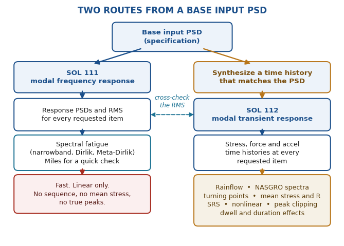
Figure 7. The two routes, and the cross-check between them.
Recommendation
Run SOL 111 first, always. It is fast, it exposes modeling errors early, it gives the RMS levels needed for screening, and it produces the response PSDs that spectral fatigue methods consume. For a component that is being checked against an allowable stress, that may be the entire analysis.
Then, if the output has to be rainflow counted, if it is going into NASGRO or any other crack growth code, if the structure has a nonlinearity that matters, if the random loads have to be combined with quasi-static loads, or if anyone needs a defensible peak rather than a habitual three-sigma multiplier, synthesize a time history that matches the specification PSD and run SOL 112. Use the SOL 111 RMS as the acceptance criterion for the SOL 112 run. If the two agree within a percent, the time history is trustworthy, and it will answer questions the PSD was never able to reach.
The frequency domain tells you how much. The time domain tells you what happened, in what order, and against what mean. Fatigue and fracture care about all three.
Related free ebooks on shock and vibration response spectra, stress-velocity, and fatigue are available at Tom’s Ebooks.
1 thought on “NASTRAN FRF & Modal Transient Analysis”