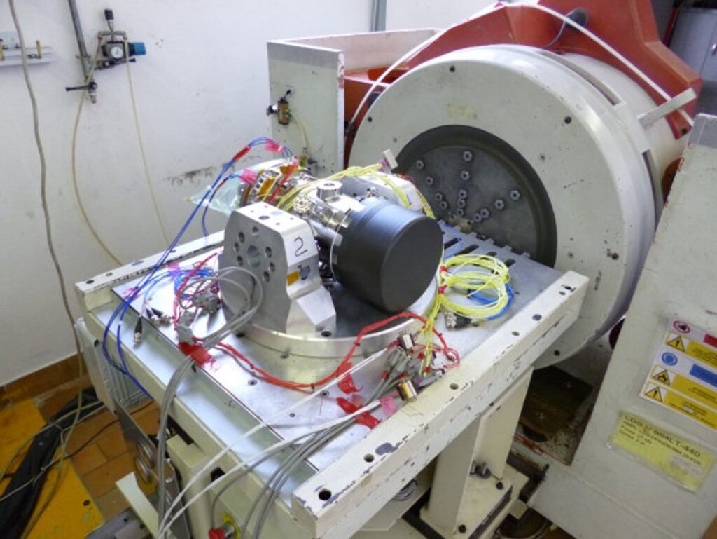
A reader sent in a question that every test engineer runs into sooner or later:
For mission synthesis we get three-axis data from the real machine. What is the best way to simulate the same thing on a single-axis shaker table to create the same vibration? Do you have any thoughts on this?
Short answer: you cannot. A single-axis shaker cannot reproduce a simultaneous three-axis environment, and no amount of clever spectrum shaping changes that. What you can do is run the three axes sequentially and then deliberately stack several conservatisms on top of the sequential test so that the test is, on balance, at least as damaging as the field. That is what the industry actually does, and it works more often than it has any right to. This post walks through the three conservatisms that do the heavy lifting, and then puts numbers on how much each one is worth.
Why Sequential Testing Is Not Equivalent
Start with the physical picture. In service, the machine drives the equipment interface in all three translations at once, plus three rotations that nobody instrumented. A weld toe, solder joint, or fillet at the critical location sees a stress that is the running sum of the contributions from every input direction, moment by moment. When two directions happen to peak together, the local stress goes higher than either direction could produce alone.
A sequential single-axis test never produces that combined peak. It produces the X contribution alone, then the Y contribution alone, then the Z contribution alone. The cycle count is right. The individual amplitudes are right. The combination is missing.
Fatigue does not care about that in a linear way. Damage goes as stress to the power $b$, where $b$ is the inverse slope of the S-N curve, roughly 3 for welds, 6 to 7 for wrought aluminum, and 9 or higher for some electronics interconnects. A modest loss of peak amplitude is a large loss of damage.
There is also a set of effects that has nothing to do with amplitude at all. Simultaneous excitation can drive modes that a single-axis input barely touches, particularly torsion and other modes with mixed participation. It produces a rotating or wandering principal stress direction, which matters for critical-plane fatigue and for anything with a directional weakness such as a lap joint or a fiber layup. It produces relative motion between neighboring items that a one-axis run cannot, so connector chafe, lead wire fretting, and cabinet-to-cabinet impact are all under-represented. Published multi-exciter comparisons have repeatedly shown specimens failing sooner under simultaneous excitation than under equivalent-level sequential single-axis excitation, and sometimes failing in a different place.
How Big Is the Deficiency? A Closed Form
Consider one critical location. Let $\sigma_X$, $\sigma_Y$ and $\sigma_Z$ be the RMS stress there from each input axis acting alone. If the three axis inputs are uncorrelated, the field stress is
$$ \sigma_{field}^2 \; = \; \sigma_X^2 + \sigma_Y^2 + \sigma_Z^2 $$Define the fraction of the mean square stress contributed by axis $i$
$$ f_i \; = \; \frac{\sigma_i^2}{\sigma_{field}^2} \, , \qquad \sum_i f_i = 1 $$Now run the sequential test with each axis at its own measured level, for the same duration as the field exposure. Using narrowband damage with a common cycle rate, the ratio of field damage to sequential test damage is
$$ R \; = \; \frac{D_{field}}{D_{test}} \; = \; \frac{1}{\sum_i f_i^{\,b/2}} $$This little formula carries most of the argument. If one axis dominates completely, $f=1$ for that axis and $R=1$. There is no deficiency, because there was nothing simultaneous to lose. The worst case is $n$ axes contributing equally, which gives
$$ R_{max} \; = \; n^{\,b/2-1} $$and the level increase needed to make it up is
$$ \Delta \; = \; \frac{20}{b}\,\log_{10} R \quad \text{dB} $$For three equally contributing axes and $b=6.4$, $R_{max}=11.2$ and $\Delta = 3.3$ dB. For two equally contributing axes at the same $b$, $R_{max}=4.6$ and $\Delta = 2.1$ dB. For welds at $b=3$ and three equal axes, $\Delta = 1.6$ dB.
That is the first useful result. The customary uncertainty factor of 3 dB is not a coincidence, and it is not merely a slush fund. It happens to be almost exactly the right size to cover the loss of simultaneity for the worst realistic case.
A Worked Example
The numbers below come from a generic demonstration model, not from any real program. A 6 kg electronics box is hard-mounted to a machine running at 1800 rpm. Triaxial acceleration was measured at the mounting interface over the mission. The three PSDs show the shaft order at 30 Hz and its harmonics, a blade-pass family, and a broadband floor that rolls off above 400 Hz.
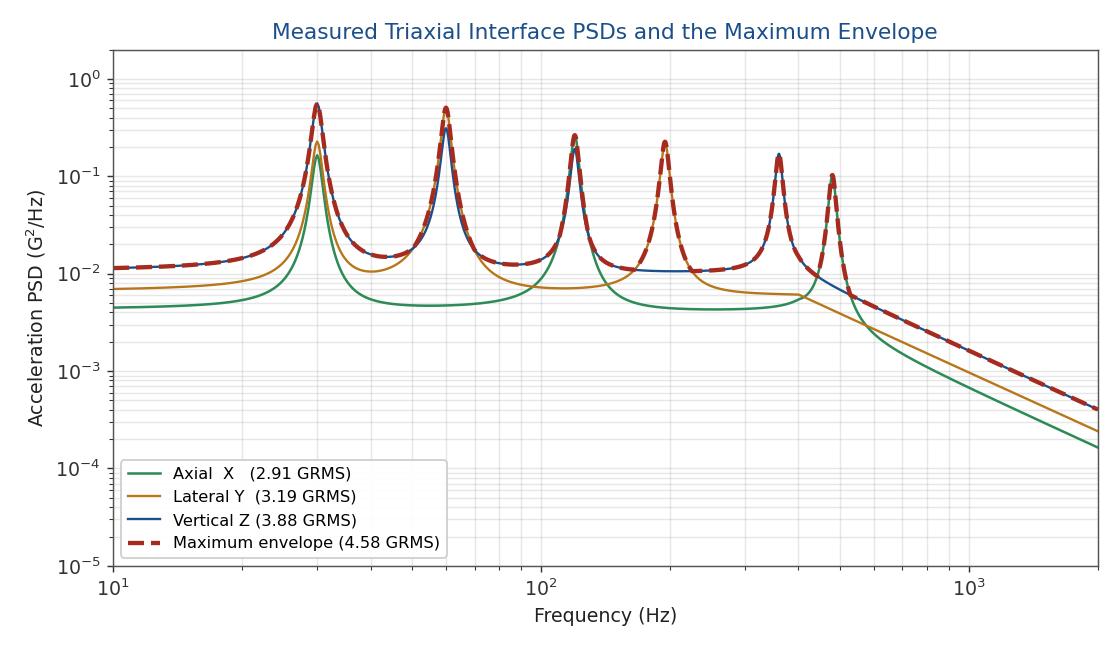
Figure 1. The three measured interface PSDs and the point-by-point maximum envelope. No single axis is the worst everywhere.
The box has one dominant mode responding to each input direction: 96 Hz driven by the axial input, 145 Hz driven by the lateral input, and 275 Hz driven by the vertical input, all with amplification near 10 to 12. Each mode delivers stress to the same critical fillet, with stress coefficients of 560, 520, and 400 psi per G of response acceleration. The choice matters, because it is the case where all three axes feed one location that produces the largest deficiency.
| Axis | Input GRMS | Box mode | Field stress, RMS | Fraction $f_i$ | Stress on envelope |
|---|---|---|---|---|---|
| Axial X | 2.91 G | 96 Hz | 2361 psi | 0.224 | 3224 psi (+2.70 dB) |
| Lateral Y | 3.19 G | 145 Hz | 2848 psi | 0.326 | 4060 psi (+3.08 dB) |
| Vertical Z | 3.88 G | 275 Hz | 3350 psi | 0.451 | 3631 psi (+0.70 dB) |
| All three at once | envelope 4.58 G | — | 4991 psi | 1.000 | — |
The fractions are 45, 33, and 22 percent, which is a realistically lopsided but still three-way split. The closed form gives $R=8.8$ at $b=6.4$, needing 2.95 dB. A full Dirlik calculation on the actual stress PSDs gives 7.5, slightly less, because the combined field stress process is broader banded and has a somewhat different peak rate than the individual axis processes. Close enough for engineering purposes, and the closed form is the one you can do in your head.
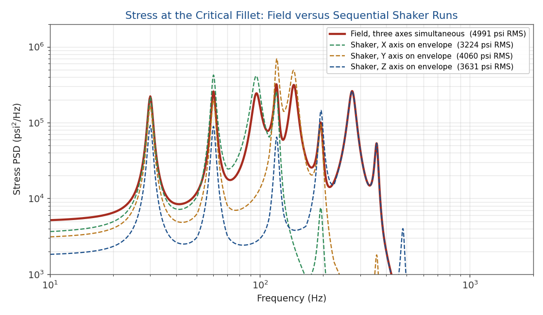
Figure 2. The field stress PSD at the critical fillet is the sum of all three contributions. Each shaker run reproduces only one of them, and none of the three individually reaches the field RMS.
Conservatism One: The Maximum Envelope of All Three Axes
The usual practice is not to test each axis at its own measured spectrum. It is to build a single test spectrum from the point-by-point maximum of all three axes, and then run that same spectrum in each of the three axes. That is the dashed red curve in Figure 1.
The justification usually offered is that it removes the risk of mislabeled or mis-oriented accelerometers, and covers the possibility that the equipment gets installed at a different orientation. Both are true. But the more important effect is the one that is rarely stated: it drags every axis up toward the worst axis, which is exactly the direction the simultaneity correction needs to go.
In this example the envelope is 4.58 GRMS against per-axis values of 2.91, 3.19, and 3.88 G. That is between 1.4 and 3.9 dB of overall input gain depending on the axis. What matters, though, is the gain at the frequency of the mode that actually loads the critical location. There the credit is smaller and unevenly distributed: 2.70 dB for the axial mode, 3.08 dB for the lateral, and only 0.70 dB for the vertical, because the vertical axis was already the highest near 275 Hz. Enveloping helps most where an axis was weak, and helps not at all where the axis was already the worst one.
That is why the envelope alone is not enough. Running the enveloped spectrum sequentially in all three axes gives 1.05 times the field damage at $b=3$, but only 0.41 times the field damage at $b=6.4$. The envelope covers the weld case and falls short of the aluminum case.
Conservatism Two: The Uncertainty dB Factor
The second step is an explicit uncertainty factor, typically 3 dB added to the enveloped PSD, sometimes 4.5 or 6 dB for qualification units or for sparse measurement sets. In the mission synthesis world this is Lalanne’s uncertainty coefficient, chosen from the statistics of the environment and the strength, and applied in the fatigue damage spectrum domain rather than to the PSD directly.
The factor is nominally there to cover measurement uncertainty, unit-to-unit variation, limited sampling of the mission, and the difference between the measurement location and the actual mounting location. It also happens to be the single cleanest way to buy back the lost simultaneity, because the required correction is a level increase and nothing else.
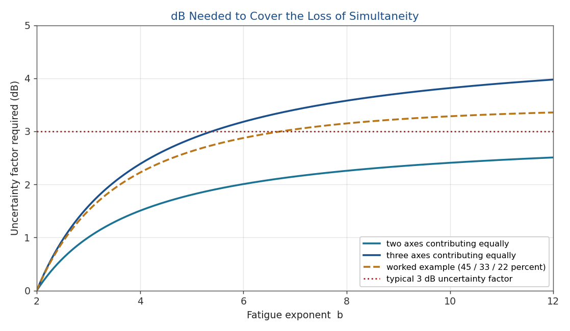
Figure 3. The level increase required to make a sequential single-axis test as damaging as simultaneous three-axis excitation, from $\Delta = (20/b)\log_{10}R$. The curves saturate, so a fixed 3 dB covers a very wide range of materials.
Figure 3 is the reassuring part of this whole discussion. The required correction saturates. Because the $20/b$ prefactor fights the growth of $R$ with $b$, the curve for three equal axes only climbs from 1.6 dB at $b=3$ to 3.8 dB at $b=10$. A flat 3 dB covers the three-equal-axis case through $b \approx 5.4$ and the worked example through $b \approx 6.8$. It covers any two-axis case out to $b=12$ with room to spare. There is no material for which 3 dB is wildly wrong, and none for which it is off by an order of magnitude in level.
In the worked example, enveloping plus 3 dB puts the sequential test at 2.97 times the field damage at $b=3$ and 3.71 times at $b=6.4$. Both are now on the conservative side.
Conservatism Three: The Rigid Fixture
The third conservatism is one nobody puts in the test plan, because it is a side effect rather than a decision. The shaker fixture is designed to be rigid to well above the test bandwidth, and the shaker with its controller is a nearly infinite-impedance source. The real mounting structure is neither.
In service, when the box goes through its fixed-base resonance, its apparent mass rises sharply and it draws reaction force from the supporting structure. The structure has finite impedance, so it yields, and the interface acceleration drops in a narrow band centered on the box resonance. That notch is physically real and it is present in the measured data, because the data was taken with the box installed.
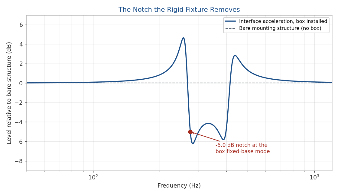
Figure 4. A two-degree-of-freedom model of a 6 kg box on a 45 kg effective mounting structure. The box unloads the structure at its own fixed-base mode, producing a 5.0 dB notch in the interface acceleration.
Then two things happen in the office. First, the notch gets erased. Straight-line breakpoints drawn through the measured spectrum, or a spectrum synthesized from an enveloped fatigue damage spectrum, will smooth right over a narrow local dip. Second, the notch cannot come back on the shaker, because the rigid fixture and the closed-loop controller will hold the commanded level at that frequency no matter how hard the test article pulls.
The result is that the test article is driven at full level through the exact frequency where the field environment gave it relief. In this example the notch is 5.0 dB deep, which raises the vertical-axis stress contribution by that amount and multiplies the sequential test damage by another factor of 1.8 at $b=3$ and 3.7 at $b=6.4$.
The Damage Ledger
Putting the whole chain together, with the field exposure normalized to 1.0.
| Test definition | Damage, $b=3$ | Damage, $b=6.4$ |
|---|---|---|
| Field, three axes simultaneously | 1.00 | 1.00 |
| Sequential, each axis at its own measured PSD | 0.63 | 0.13 |
| Sequential, maximum envelope in each axis | 1.05 | 0.41 |
| Envelope plus 3 dB uncertainty factor | 2.97 | 3.71 |
| Plus rigid fixture, notch not restored | 5.34 | 13.54 |
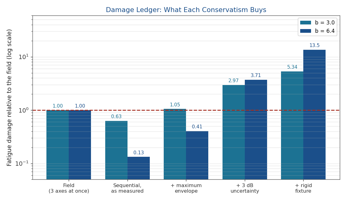
Figure 5. Fatigue damage relative to the field exposure, log scale. The bare sequential test under-tests badly at high $b$. The stack of conservatisms recovers it and then some.
The pattern is worth memorizing. The bare sequential test under-tests, and it under-tests worst for exactly the materials where fatigue calculations are most sensitive. The maximum envelope roughly cancels the deficiency at low $b$ and only partly cancels it at high $b$. The 3 dB uncertainty factor is what actually crosses the line. The rigid fixture then adds a bonus that is welcome up to a point and dangerous past it.
What the Conservatism Does Not Buy
Level margin fixes an amplitude problem. It does not fix a kinematics problem, and it is important to be clear about the difference.
The ledger above is built for one critical location fed by all three axes. If different axes drive different critical locations, each location only ever sees one axis, $f=1$ for that location, and the simultaneity deficiency vanishes. Conversely, if the three input axes are correlated rather than independent, which is common on machinery where a single unbalance drives everything, the root-sum-square combination is wrong and the true field stress can be higher still.
Beyond that, a sequential test with extra level does not reproduce a rotating principal stress direction, does not produce the relative motion between adjacent items that causes chafe and fretting, does not correctly load rotational degrees of freedom at the interface, and does not excite modes whose participation requires two directions at once. Nor does level margin help with rattle, chatter, intermittent contact, or anything else that is a displacement or a clearance phenomenon rather than a stress phenomenon. If your dominant concern is one of those, more decibels will not save you.
There is also a cost to over-testing. A test at 13 times the field damage will occasionally fail hardware that would have flown for twenty years, and the redesign that follows is real money spent on a phantom. Track the margin. Do not let it stack silently.
A Practical Recipe
For mission synthesis from triaxial field data to a single-axis shaker test:
- Process each measured axis separately over the full mission. Compute a fatigue damage spectrum and an extreme response spectrum per axis, using the $b$ exponent and $Q$ appropriate to the hardware. Do not average the axes and do not vector-sum the accelerations.
- Take the point-by-point maximum of the three fatigue damage spectra, and separately of the three extreme response spectra. Envelope in the damage domain rather than the PSD domain if you have the tools, since that is where the duration compression is done consistently.
- Apply the uncertainty factor. Three decibels is the common default and, as shown above, is close to the right size for the simultaneity deficiency alone. Consider more if the mission sampling was thin or the measurement location was remote from the mounting interface.
- Synthesize the test PSD for the compressed test duration and check it against the extreme response spectrum so that the accelerated test does not exceed yield or peak-limited allowables while matching damage.
- Run that one spectrum in all three orthogonal axes, full duration in each. Total damage delivered is the sum over the three runs.
- Before the test, estimate the impedance mismatch. Compare the apparent mass of the test article at its first mode against the driving-point apparent mass of the real mounting structure. If the mismatch implies more than about 6 dB of accidental over-test, plan for force limiting and instrument the interface with force gages or an equivalent measurement.
- Document the whole margin stack in the test plan. The reviewer three years from now needs to know that the 3 dB was doing double duty.
When to Stop Compensating and Buy the Right Test
Sequential single-axis testing with enveloping and an uncertainty factor is the right answer for the large majority of equipment. It is cheap, repeatable, universally understood, and demonstrably conservative for fatigue.
Push for multi-exciter testing when the failure mode is not fatigue at a single location. MIL-STD-810 Method 527 covers multi-exciter testing and is the natural reference. Good candidates include articles with strong torsional or mixed-participation modes, assemblies where relative motion between components is the concern, structures with clearances and potential impact, composite or bonded joints with directional weakness, and anything where a previous single-axis qualification passed and the fielded hardware failed anyway. That last one is the clearest signal that the surrogate has stopped working.
Also push back the other way. If your item is genuinely single-axis dominated, with one $f_i$ above about 0.8, then the closed form says $R$ is barely above 1 and you are stacking margin against a deficiency that does not exist. Compute $f_i$ before you accept the default.
Free ebooks on shock and vibration response spectra, stress-velocity, fatigue, and related topics are available at Tom’s ebooks.
Questions and corrections are welcome, as always.