Dynamic Versus Static Modulus: Why ASTM E1876 and ASTM E111 Don’t Always Agree
Engineers frequently encounter situations where material properties reported in handbooks don’t quite match experimental data. A classic example occurs when comparing elastic modulus values obtained from different test standards.
When evaluating stiffness, two common benchmarks—ASTM E1876 (Dynamic/Impulse Excitation) and ASTM E111 (Static Tension/Compression)—frequently yield different numbers for the exact same material. Understanding why they disagree is critical for accurate structural dynamics, finite element analysis (FEA), and materials characterization.
The Core Difference
ASTM E1876-22 uses impulse excitation—a small mechanical hammer strike—and measures the resulting resonant frequencies of a specimen via an acoustic microphone or laser vibrometer. Young’s modulus is then back-calculated from these resonant frequencies, the specimen’s precise geometry, and its mass. This is inherently a small-strain, high-strain-rate measurement.
By contrast, static modulus measurements, such as ASTM E111 tension or compression testing, determine the stress-strain slope under slow, sustained loading using a traditional universal testing machine. This method captures a large-strain, low-strain-rate response where microcracking, viscoelastic creep, stress relaxation, and other inelastic effects have time to develop.
Because they probe fundamentally different physical regimes, the dynamic modulus is almost universally higher than the static modulus.
Quick-Reference Comparison
| Feature / Parameter | ASTM E1876 (Dynamic / Impulse) |
ASTM E111 (Static / Quasi-Static) |
|---|---|---|
| Primary Loading Mechanism | Mechanical impulse (transient impact) | Continuous, slow uniaxial loading |
| Strain Rate (\(\dot{\varepsilon}\)) | Very High (\(1\text{e}1\) to \(1\text{e}3 \text{ s}^{-1}\)) |
Very Low (\(1\text{e}\text{-}5\) to \(1\text{e}\text{-}3 \text{ s}^{-1}\)) |
| Strain Amplitude (\(\varepsilon\)) |
Microstrain (\(\le 1\text{e}\text{-}6\)) |
Macrostrain (\(1\text{e}\text{-}4\) to \(1\text{e}\text{-}2\)) |
| Inelastic Effects Captured | Purely elastic response, phase lag | Creep, relaxation, microcracking, plasticity |
| Outputs Obtained | Storage modulus (\(E’\)), Loss factor (\(\eta\)) |
Tangent or Secant Young’s Modulus (\(E\)) |
For common engineering metals, the difference is modest—often only 1–5%—and structural dynamics practitioners frequently ignore it without introducing significant error. However, for concrete, ceramics, rock, and especially polymer-matrix composites, the gap can be massive and will significantly affect analysis results.
An additional distinction is strain amplitude. Impulse excitation testing is performed at extremely small strain levels, typically deep in the microstrain range. Many materials exhibit stiffness degradation as strain amplitude increases. Consequently, part of the dynamic-static modulus difference arises from strain-amplitude effects rather than loading rate alone. This phenomenon is particularly important for concrete, rock, soils, filled polymers, and some composite systems.
When It Actually Matters
For metallic structures operating in the typical structural vibration range (roughly 1 Hz to 2 kHz), using the static modulus from a handbook is generally adequate for eigenvalue analysis. The resulting error is usually smaller than uncertainties associated with geometry, boundary conditions, joint stiffness, and manufacturing variability.
The situation changes under several important circumstances.
Polymer-Matrix Composites and Elastomers
Viscoelastic materials exhibit stiffness that depends heavily on both frequency and temperature. A single, static modulus value is therefore only an approximation.
Dynamic Mechanical Analysis (DMA) provides the storage modulus \(E'(\omega)\) and loss modulus \(E”(\omega)\) as continuous functions of frequency (\(\omega\)). This frequency-dependent representation is generally the appropriate framework for simulating viscoelastic materials.
Concrete and Rock: The Microcracking Threshold
Dynamic moduli for concrete commonly exceed static values by 20–40%, and similar behavior is observed in many geological materials.
Static testing (ASTM E111) allows time for microcracks at the interfacial transition zone (ITZ) between aggregate and cement paste to propagate and open, artificially softening the macroscopic stress-strain slope. Because ASTM E1876 operates at microstrain amplitudes, it probes the material well below this damage threshold, capturing the uncracked, pristine matrix stiffness. For seismic analysis, blast loading, acoustic response, and vibration prediction, this difference becomes a first-order effect.
High-Frequency Response and Wave Propagation
At frequencies above approximately 1–2 kHz, dynamic material properties become increasingly important. The response begins to reflect local material behavior and wave propagation characteristics rather than simple global structural modes.
Because bulk longitudinal wave speed scales as:
\[c = \sqrt{\frac{E}{\rho}}\]
and bending (flexural) wave speeds scale non-linearly with \(\sqrt[4]{E}\), even a modest increase in modulus produces measurable changes in longitudinal-wave speed, bending-wave speed, transmission efficiency, and acoustic radiation behavior. For applications such as structure-borne noise, acoustic fatigue, Statistical Energy Analysis (SEA), and ultrasonic testing, dynamically measured properties are the correct choice.
Damping Estimation
ASTM E1876 provides more than modulus. By analyzing the ring-down decay after an impulse excitation, it yields material damping expressed as a loss factor (\(\eta\)). Static tests provide essentially no damping information. If forced-response prediction near resonance is required, the dynamic loss factor obtained from ASTM E1876 is often more valuable than the modulus itself.
Modal Correlation and Finite Element Models
Engineers performing experimental modal analysis encounter this issue routinely. During finite-element model correlation, Young’s modulus is often treated as a tuning parameter. The modulus that best matches measured natural frequencies frequently ends up closer to the dynamic modulus than to the handbook static value.
As a result, analysts commonly observe that a model correlates most accurately when the effective modulus is a few percent higher than the nominal static value reported in material handbooks. This observation is not necessarily evidence of modeling error. Rather, it reflects the fact that modal testing and resonance measurements probe the material under dynamic, small-strain loading conditions.
⚠️ Crucial FEA Pitfall: Modulus Tuning vs. Mass Density
When treating Young’s modulus as a tuning parameter during modal correlation, analysts must remember that resonant frequencies scale as \(\omega \propto \sqrt{E/\rho}\). If a model’s frequencies are off by 3%, increasing \(E\) by 6% might fix the frequency match, but it could easily mask a poorly modeled boundary condition or an incorrect non-structural mass distribution. Only lean into the dynamic modulus shift if your geometry and mass matrices are definitively verified.
Hysteresis and Complex Moduli
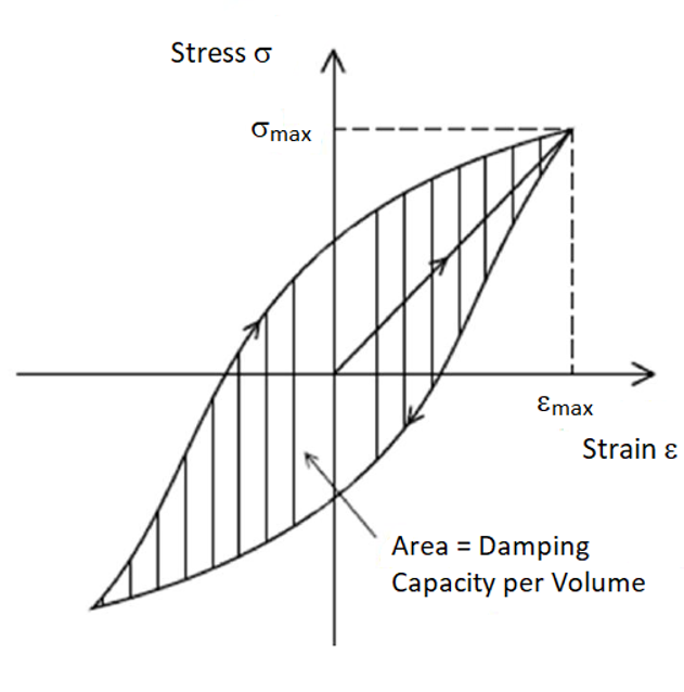
When a viscoelastic material is subjected to cyclic loading, the stress-strain curve traces a closed loop rather than a straight line. That loop is hysteresis.
The enclosed area represents energy dissipated during each cycle of loading and unloading. A perfectly elastic material exhibits no hysteresis loop. A purely viscous material produces a maximally open loop. Real engineering materials fall somewhere between these two extremes.
The complex modulus formulation captures this behavior directly:
\[E^* = E’ + iE”\]
where:
- \(E’\) = storage modulus (energy-storing component)
- \(E”\) = loss modulus (energy-dissipating component)
The ratio of these quantities defines the material loss factor:
\[\eta = \frac{E”}{E’}\]
In DMA literature, the same quantity is commonly expressed as \(\tan \delta\), where \(\delta\) is the phase angle between stress and strain.
- For lightly damped metals, \(\tan \delta\) is typically between 0.001 and 0.01.
- For filled elastomers, viscoelastic damping layers, and polymeric materials, \(\tan \delta\) may range from 0.5 to 1.5 or even higher, depending on frequency and temperature.
Connection to ASTM E1876
The connection between ASTM E1876 and complex modulus theory is direct. The measured resonant frequency provides the storage modulus \(E’\), while the ring-down decay provides the loss factor \(\eta\). Thus, a single impulse excitation test provides both stiffness and damping information from a small specimen.
One important limitation is that ASTM E1876 measures these quantities only at the specific natural frequencies of the test specimen. It does not provide a continuous frequency-dependent characterization. For a complete description of \(E'(\omega)\) and \(E”(\omega)\) over a broad frequency range, DMA testing is required, often paired with time-temperature superposition to extend the effective frequency range by several decades.
Furthermore, the loss factor extracted from ASTM E1876 is associated with a specific resonant mode. In materials exhibiting frequency-dependent damping, different resonances may produce different apparent loss factors. Consequently, a single measured value of \(\eta\) should not automatically be assumed valid across all frequencies.
Implications for Finite Element Analysis
In frequency-domain analysis, complex modulus enters naturally through the complex stiffness matrix:
\[K^* = K(1 + i\eta)\]
This represents the structural damping, or hysteretic damping, model, which assumes that \(\eta\) remains constant with frequency. For metals, this approximation is often reasonable. For polymers and viscoelastic materials, it is usually poor because damping and stiffness vary substantially with frequency and temperature.
When modeling constrained-layer damping treatments, elastomeric mounts, or potting compounds, frequency-dependent complex moduli should be used. Many commercial solvers support such formulations through frequency-dependent material properties.
One caution deserves emphasis: The structural damping model behaves well in the frequency domain but is formally non-causal in the time domain. Consequently, transient analyses generally rely on viscous damping formulations using a damping matrix \(C\) rather than a frequency-independent complex stiffness model. This distinction becomes critical when both frequency-domain and time-domain simulations are performed on the same structure.
Special Considerations for Composites
For isotropic materials, a single Young’s modulus often provides an adequate description of stiffness. Composite laminates are different.
The modulus obtained from ASTM E1876 depends heavily on specimen geometry, fiber layup, and the selected vibration mode. A flexural resonance primarily reflects bending stiffness in the dominant material direction and may not uniquely identify all elastic constants required for a complete orthotropic material model (such as Poisson’s ratios and shear moduli).
Therefore, while ASTM E1876 provides valuable dynamic property data for composites, additional testing configuration orientation or static testing is often necessary to isolate the full set of orthotropic engineering constants used in shell or solid FEA elements.
Practical Recommendations
For metal structures involved in conventional vibration analysis—such as modal surveys, FRF correlation, sine testing, random vibration, and most aerospace or machinery applications—the static modulus from ASTM E111 or material handbooks is generally adequate.
ASTM E1876 becomes particularly valuable when:
- Material volume is limited: Modulus and damping must be obtained from the same small, simple test coupon.
- High-temperature screenings are needed: ASTM E1876 requires no mechanical grips, extensometers, or load frames inside the hot zone (only acoustic or optical paths), making it exceptionally well-suited for measuring modulus degradation of ceramics and superalloys up to and beyond 1000°C.
- The material is highly strain-rate sensitive: The application involves concrete, rock, deep-set polymers, or advanced composites.
- High-frequency acoustics are involved: High-frequency SEA, acoustic fatigue, or wave-propagation analyses require dynamic wave-speed accuracy.
Final Perspective
The question is not whether the dynamic modulus is “more correct” than the static modulus. Each represents the material under a completely different physical regime.
The appropriate modulus is the one measured under conditions that most closely resemble the intended application in terms of strain amplitude, loading rate, frequency, and temperature. For many metal structures, the distinction is small enough to ignore. For viscoelastic materials, composites, concrete, rock, and high-frequency acoustic applications, it can become one of the dominant factors governing the accuracy of analysis and test correlation.
– Tom Irvine