A colleague who has started building a simulator wrote in with a short question. He has welded rods in S355 or S420 steel, the welding process is not yet fixed, and he expects that a fatigue assessment will be needed. He has not worked with welded rods before, and his working assumption was that they would behave much like the parent material, only worse. How should he proceed?
That working assumption is the one I want to evaluate first, because it is the single most common misconception about welded joints, and it is the reason a lot of welded machinery frames crack in service long before anyone expected them to.
The Short Answer
A welded joint is not the parent material with a knockdown factor. It is a different fatigue problem with a different governing variable. The fatigue strength of an as-welded joint is set almost entirely by the local geometry of the weld and the quality of the weld, and it is very nearly independent of the strength of the steel you welded. S355 and S420 give the same welded fatigue life. Choosing the higher grade buys you static capacity, and it buys you nothing at all in the as-welded condition.
The governing rule. For as-welded joints in structural steel, the design S-N curve depends on the joint geometry, not on the yield or tensile strength of the base metal. All of the major codes are written this way: EN 1993-1-9, the IIW Recommendations, AWS D1.1, DNV-RP-C203, and BS 7608. There is no grade term in any of them.
So the answer to “how do I proceed” is: stop thinking in terms of a material S-N curve with a stress concentration factor, and start thinking in terms of detail categories. You classify each weld by its geometry, you look up the design curve for that class, you compute a nominal or structural stress in the member, and you accumulate damage against that curve.
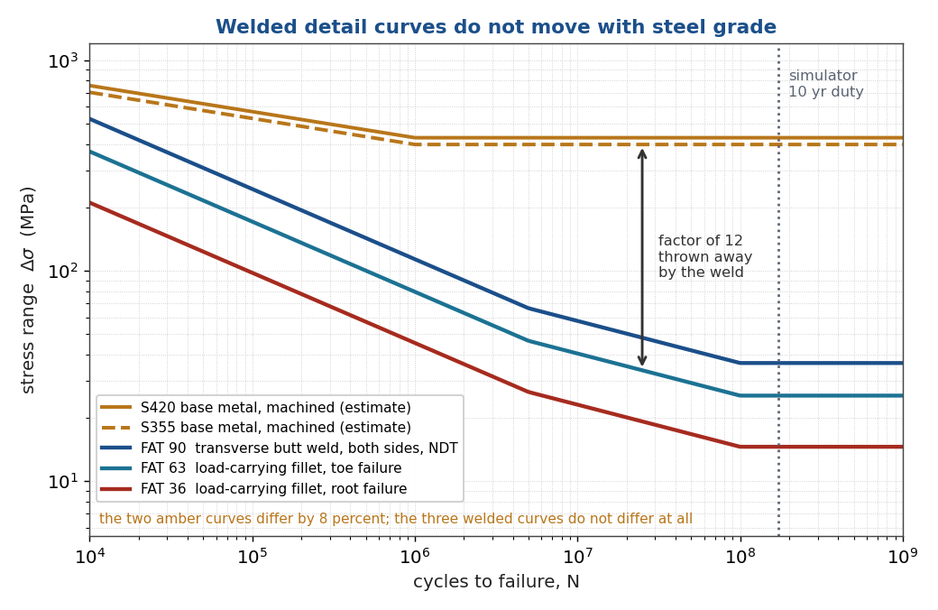
Figure 1. The two base metal curves are 8 percent apart. The three welded curves are the same curves for both grades, because the code does not contain a grade term. At a hundred million cycles the weld has thrown away roughly a factor of twelve.
Why the Grade Drops Out
Three mechanisms conspire, and each of them is insensitive to base metal strength.
The weld toe is already a crack. Fatigue life in unwelded metal is dominated by crack initiation, which is the part of the process that scales with strength and surface finish. A weld toe contains intrusions, undercut, slag inclusions and non-metallic particles on the order of 0.05 to 0.4 mm deep. The initiation phase is effectively already spent when the part leaves the fabrication shop. What remains is propagation, and propagation in ferritic steels is governed by the Paris law, whose constants are essentially the same for S235 as for S690.
Residual stress swallows the mean stress. Welding leaves tensile residual stresses at the toe that approach the yield strength of the material. The consequence is that the local stress cycle runs down from yield regardless of what the applied mean stress is. This is why the codes tell you to use the full stress range with no mean stress correction for as-welded joints, and it is also why a higher yield strength is no help: a stronger steel simply locks in a larger residual stress. Goodman and Gerber corrections do not belong in an as-welded assessment.
Notch sensitivity rises with strength. Even setting the other two aside, higher strength steels are more notch sensitive, so the fraction of the plain-material improvement that survives into a notched detail keeps shrinking. The net effect across the three mechanisms is that the measured scatter bands for welded joints in mild and high strength steel overlap almost completely.
Detail Categories and the Design Curve
The detail category, written FAT 63 in IIW notation or “detail category 63” in Eurocode notation, is the characteristic stress range in MPa that the detail survives for two million cycles, at a 95 percent survival probability with 75 percent confidence. Everything else follows from that one number.
EN 1993-1-9 uses a trilinear curve. Above the knee the slope is $m=3$:
$$N = 2\times10^{6}\left(\frac{\Delta\sigma_C}{\Delta\sigma}\right)^{3}$$
The constant amplitude fatigue limit sits at five million cycles,
$$\Delta\sigma_D=\Delta\sigma_C\left(\frac{2}{5}\right)^{1/3}=0.737\,\Delta\sigma_C$$
and below it the slope flattens to $m=5$ down to a cut-off limit at a hundred million cycles,
$$\Delta\sigma_L=\Delta\sigma_D\left(\frac{5}{100}\right)^{1/5}=0.549\,\Delta\sigma_D=0.405\,\Delta\sigma_C$$
The IIW Recommendations use the same idea with different numbers: the knee sits at ten million cycles, the second slope is $m=5$ from Haibach’s rule, and there is no hard cut-off until a billion cycles. For a machine that accumulates a hundred million cycles or more, the difference between these two tails is not academic. It is most of the answer.
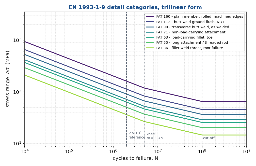
Figure 2. The detail category family. Selecting the right curve is a geometry and quality decision, not a materials decision.
Here are the categories most likely to be relevant to a welded rod. Treat these as representative values to orient yourself; the governing numbers are in the tables of whichever code you are working to, together with their execution requirements, and those requirements are part of the class.
| Detail | Typical FAT | Notes |
|---|---|---|
| Plain member, rolled, machined edges | 160 | The unwelded reference. No weld anywhere near the section. |
| Transverse butt weld, ground flush, full NDT | 112 to 125 | The best a weld gets. Grinding must be parallel to the stress direction. |
| Transverse butt weld, as welded, both sides, NDT | 80 to 90 | Requires a controlled toe angle and proven root quality. |
| Butt weld from one side, no backing | 63 to 71 | The root is now the critical location and it is hard to inspect. |
| Non-load-carrying transverse attachment | 71 to 80 | A bracket, a lug, a gusset that does not carry the member force. |
| Load-carrying fillet or partial penetration joint, toe failure | 63 | The workhorse case for a rod welded into a gusset or a node. |
| Longitudinal attachment, length dependent | 50 to 71 | Falls with attachment length. A long stiffener is worse than a short one. |
| Threaded rod, rolled thread, tension | 50 | Cut threads are worse. Also independent of grade. |
| Fillet weld throat, root failure, throat stress | 36 to 40 | Assessed on stress in the throat area, not on member stress. |
Note the range. From the unwelded reference at 160 down to a fillet weld root at 36 is a factor of 4.4 in stress and a factor of 86 in life at $m=3$. That is the design space you actually control. The grade change from S355 to S420 does not appear anywhere in it.
Which Stress Goes Into the Curve
This is where people go wrong with finite element models. The detail categories were derived from tests in which the reported stress was the nominal stress, computed by beam theory over the gross section, with the weld notch excluded. If you build a fine shell or solid mesh, read off the peak stress at the toe, and compare it to FAT 63, you will double count the notch and get an answer that is wrong by a factor of two to four.
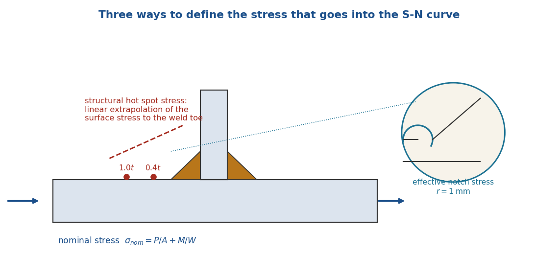
Figure 3. Each stress definition has its own family of S-N curves. Mixing a stress from one column with a curve from another is the most common error in welded fatigue analysis.
There are three consistent pairings, and you must stay inside one of them.
Nominal stress with the detail category tables. Compute $\sigma = P/A + M/W$ in the member, away from the weld. Use beam elements or hand calculations. This is the right choice when your geometry matches a tabulated detail, which is usually the case for a rod in a frame.
Structural hot spot stress with FAT 90 or FAT 100. Compute the surface stress at 0.4 times the thickness and 1.0 times the thickness away from the toe, then extrapolate linearly to the toe. This captures the gross geometry and the misalignment but deliberately excludes the weld notch itself, which the S-N curve already contains. Shell elements sized at the plate thickness work well; the mesh must be regular near the extrapolation points. Use this when the geometry is not in the tables, which is common at a tubular node.
Effective notch stress with FAT 225. Model the toe and the root with a fictitious 1 mm radius, mesh at $r/6$ or finer, and read the peak. Expensive, and only worth it when you need to compare candidate weld geometries or when you must assess a root that has no tabulated class.
Does the Undefined Welding Process Matter?
Less than you would think, and more than you would like.
The detail categories are process independent. MAG, stick, TIG and submerged arc all land on the same curve if the finished geometry and quality are the same. So not having settled the process is not, by itself, a blocker for starting the assessment.
What you cannot defer is the quality specification, because the class you assume in analysis is only real if the shop delivers it. Four things carry almost all of the risk, and each of them needs to appear on the drawing:
- Penetration. A partial penetration joint that you analyzed as full penetration is not a conservative approximation. It is a different failure mode at a much lower class, initiating at a root you cannot inspect.
- Toe geometry. Undercut and a steep toe angle push a FAT 90 detail down toward FAT 63 or below.
- Misalignment. Axial and angular misalignment generate secondary bending. More on this below.
- Start and stop positions. On a circumferential weld around a rod, the overlap at the closure is a classic initiation site. Specify where it goes, and keep it away from the peak stress location.
ISO 5817 quality levels B, C and D are the usual vehicle, but be aware that those levels were written around weldability and general workmanship, not around fatigue. Roughly speaking, level D supports only the lower categories, level C the middle range, and level B or better is the price of admission for the higher ones. For the fatigue-critical imperfections you should call out the acceptance criteria explicitly rather than relying on the level alone.
The root is a crack you built on purpose. A rod fillet welded into a plate or a gusset without full penetration has an unfused interface at the root that behaves as a pre-existing planar crack. No NDT method finds it, because it is supposed to be there. If the load path drives the root rather than the toe, you are at FAT 36 to 40 assessed on the throat area, which is the lowest class in the table. On a solid round bar this deserves particular attention, because the crack front sweeps around the circumference with no alternate load path and no redistribution.
Mean Stress, Misalignment and Thickness
Mean stress. For as-welded joints, use the full stress range and apply no mean stress correction. A bonus factor is available for stress-relieved joints and for base material in complete compression, but for a welded frame in the as-welded condition the factor is 1.0. This is one of the rare simplifications welding gives you.
Misalignment. Any eccentricity between the two pieces you joined turns axial load into bending. For a solid round bar of diameter $d$ with eccentricity $e$, the free-body ratio of bending stress to membrane stress is
$$\frac{\sigma_b}{\sigma_m}=\frac{8e}{d}$$
so the magnification factor is $k_m=1+8e/d$ in the unrestrained case. Restraint from the surrounding structure reduces this, often to about half. The tabulated detail categories already contain an allowance for a modest amount of misalignment, of order $e/t=0.1$ for butt joints, so apply $k_m$ only for the excess. Even so, the numbers are sobering.
| $e/d$ | $k_m$ free | $k_m$ half restrained | Life factor at $m=3$ |
|---|---|---|---|
| 0.02 | 1.16 | 1.08 | 0.64 to 0.79 |
| 0.05 | 1.40 | 1.20 | 0.36 to 0.58 |
| 0.10 | 1.80 | 1.40 | 0.17 to 0.36 |
| 0.20 | 2.60 | 1.80 | 0.06 to 0.17 |
A two millimetre offset on a 20 mm rod costs somewhere between two thirds and five sixths of the fatigue life. That is a fit-up and jigging problem, not an analysis problem, and it is worth solving on the shop floor rather than in the spreadsheet.
Thickness. The categories are referenced to 25 mm. For thicker sections a size correction applies with an exponent of roughly 0.1 to 0.3 depending on the detail. For a thin rod there is no bonus in the codes, so do not take one.
Variable Amplitude and the Cycle Count Problem
A simulator is not a bridge. A bridge sees a few million significant cycles in a century. A motion platform running eight hours a day, three hundred days a year, for ten years, with an effective significant cycle rate of two per second, accumulates
$$N = 24{,}000 \text{ h} \times 3600 \text{ s/h} \times 2 \text{ Hz} = 1.73\times10^{8} \text{ cycles}$$
That is two orders of magnitude beyond the reference point of the S-N curve. It puts you out on the shallow tail of the curve where the code writers had the least data and where the codes disagree with each other most. It also means the constant amplitude fatigue limit is not a hiding place: with a broadband random stress history, some cycles always exceed it, and once they do, the whole spectrum becomes damaging.
The mechanics are standard. Rainflow count the stress history, or the stress power spectral density if you are working in the frequency domain, and accumulate damage by Palmgren-Miner:
$$D=\sum_i \frac{n_i}{N_i}\le D_{lim}$$
Two points on the accounting. First, the IIW recommends $D_{lim}=0.5$ for welded joints under variable amplitude loading, not 1.0, and 0.2 if the mean stress itself fluctuates. Second, when any cycle exceeds the knee, use the Haibach slope of $m=5$ below the knee rather than truncating. If you truncate at the constant amplitude limit, you will predict infinite life for a joint that is quietly cracking.
If your input is a PSD rather than a time history, the spectral methods apply directly. Dirlik is the usual choice for a bilinear curve; the narrowband approximation is conservative for broadband response and can be badly so. I have written elsewhere about the correction factors between narrowband, Dirlik and rainflow damage, and about the Meta-Dirlik refinement, and all of that carries over to welded details without change. The only thing that changes is which S-N curve you feed it.
A Worked Example
Take a diagonal brace in a welded platform frame, a circular hollow section 60.3 mm outside diameter with a 5.0 mm wall. The area is 869 mm² and the elastic section modulus is 11.1 cm³. The duty cycle is the one above, $1.73\times10^{8}$ cycles. Assume the axial stress in the brace is narrowband with Rayleigh distributed peaks, and solve for the RMS nominal stress that exactly consumes $D=0.5$ using the EN 1993-1-9 trilinear curve.
| Detail | FAT | $\Delta\sigma_D$ (MPa) | $\Delta\sigma_L$ (MPa) | Allowable RMS (MPa) | RMS axial force (kN) |
|---|---|---|---|---|---|
| Butt weld, as welded, NDT | 90 | 66.3 | 36.4 | 8.5 | 7.4 |
| Load-carrying fillet, toe | 63 | 46.4 | 25.5 | 5.9 | 5.2 |
| Fillet weld root, throat stress | 36 | 26.5 | 14.6 | 3.4 | 2.9 |
Read the middle row again. The allowable RMS nominal stress at a load-carrying fillet weld is 5.9 MPa. The yield strength of the S355 you would build it from is sixty times that number. For S420 the ratio is seventy one, which is the whole story in one line: the higher grade makes the ratio worse, not better, because you will be tempted to size the member for static strength and then discover that fatigue governs by a factor of sixty.
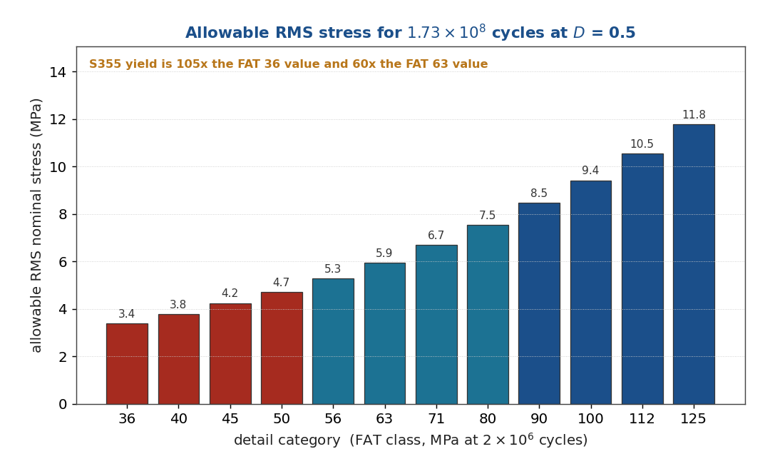
Figure 4. Allowable RMS nominal stress across the detail categories for the simulator duty cycle. The entire chart fits inside the bottom four percent of the yield strength.
Before anyone concludes that welded machinery frames cannot be built, note the assumption doing the most work here: a stationary narrowband process running at full amplitude for every operating second. Real duty cycles spend most of their time at low amplitude, and the total damage is very sensitive to that distribution. This is precisely why the assessment has to be driven by a measured or simulated load spectrum rather than by an assumed RMS level. Figure 5 shows how the allowable moves with the cycle count, which is the same sensitivity seen from a different angle.
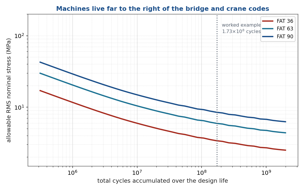
Figure 5. Allowable RMS nominal stress versus accumulated cycles. Getting the duty cycle wrong by a factor of ten costs roughly 35 percent of the allowable stress.
The Trap Specific to Welded Frames
There is one more issue that catches people building welded space frames, and it has nothing to do with the weld metal.
Frames like this are usually analyzed as trusses, with pinned joints and axial members only. Welded nodes are not pins. They are rigid, and rigid nodes generate secondary bending moments in the members that a truss model does not report at all. In a stiff welded frame the secondary bending stress at the node can equal or exceed the axial stress, and it peaks exactly where the weld toe is. A truss analysis that says the brace carries 5 kN axial and nothing else can be understating the stress range at the critical toe by a factor of two or more.
Model the frame with beam elements and rigid connections. Include the joint eccentricities, meaning the offsets between member centrelines at the node. If the node is a tubular joint with a brace welded onto a chord, the local chord wall flexibility raises the hot spot stress further, with stress concentration factors commonly in the range of two to six; CIDECT Design Guide 8 and the DNV hot spot approach cover that case properly and it is worth using them rather than guessing.
What Actually Buys You Life
Since the grade does not, here is what does, roughly in order of return on effort.
Move the weld. The cheapest fatigue improvement in existence is to put the joint where the stress range is low. A weld at an inflection point costs nothing. A weld at the peak moment costs everything.
Change the detail class. Going from a partial penetration fillet to a full penetration butt weld with a ground toe moves you from FAT 36 or 63 up toward FAT 90 or 112. At $m=3$ that is a factor of 5 to 30 in life for the price of a better joint preparation and an NDT line item.
Grind the toe. Burr grinding or TIG dressing typically buys around 30 percent in stress, which is roughly a factor of two in life. The grinding must remove the intrusions, which means going about 0.5 mm below the original surface, and it must run parallel to the load direction.
Treat the toe by high frequency mechanical impact. This is the one place where the grade finally pays. HFMI introduces compressive residual stress and improves the toe profile, and the IIW recommendations grant the benefit as a function of yield strength: four fatigue classes for steel at or below 355 MPa, and one more class for each further band. S355 gets four classes, a factor of 1.58 in stress. S420 gets five classes, a factor of 1.78. That is a real 13 percent advantage for the higher grade, and it exists only because of the treatment.
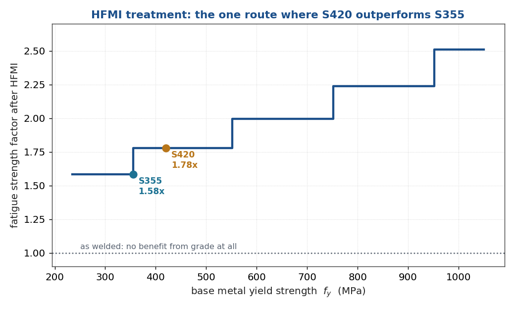
Figure 6. HFMI benefit as a function of base metal yield strength. The as-welded line at 1.0 is flat across the whole range; that flatness is the point of this article.
Two cautions on HFMI. The benefit is fully available only at low stress ratio; it is reduced progressively as the mean stress rises, and above roughly $R=0.4$ no improvement can be claimed without testing. And the treatment is only as good as its quality control, so it needs a procedure and an inspection criterion like any other process.
Do not weld at all where it matters most. For the highest-cycle load paths in a simulator, consider bolted or pinned connections with spherical rod ends. A machined and rolled-thread rod end at FAT 50 or better, with a defined preload, is often a more predictable fatigue detail than a welded node at FAT 63, and it is inspectable and replaceable.
A Procedure
- Define the duty cycle first. Hours per day, days per year, design life, and the load spectrum. This drives everything and it is the input with the largest uncertainty. Get a measured or simulated load history if you can.
- Build a beam element model with rigid nodes and real eccentricities. Extract member force and moment time histories, or PSDs, at every welded location.
- Classify every weld. Walk the drawing joint by joint and assign a detail category to each one, with the geometry and quality requirements that go with it. Where nothing fits, go to hot spot stress.
- Check for a root-critical load path at every partial penetration joint, and assess it on throat stress separately from the toe.
- Apply the magnification factors for misalignment beyond the built-in allowance, and for thickness if applicable.
- Rainflow count and accumulate damage with the Haibach slope below the knee and $D_{lim}=0.5$. Use the full stress range with no mean stress correction.
- Apply the partial factor. EN 1993-1-9 gives $\gamma_{Mf}$ from 1.00 to 1.35 depending on whether the assessment is damage tolerant or safe life, and on the consequence of failure. A simulator with a person inside it is a high consequence, safe life structure. That is the 1.35 column.
- Instrument and verify. Strain gauge the two or three worst joints, run a representative duty cycle, and compare the measured spectrum to the assumed one. Place gauges for hot spot extrapolation at 0.4t and 1.0t from the toe, never at the toe itself.
- Write an inspection plan. Fatigue analysis of welded structures carries scatter of a factor of two to three in stress even when everything is done correctly. Periodic inspection at the classified details is not an admission of failure; it is part of the design.
If you take one thing away. Your intuition that a welded rod behaves like the parent material but worse leads to the wrong design decisions, because it implies the fix is a better material. The fix is a better joint. Spend the budget on penetration, fit-up, toe geometry, weld location and inspection, and specify the cheapest grade that satisfies the static and buckling checks.
References and Further Reading
- EN 1993-1-9, Eurocode 3: Design of Steel Structures, Part 1-9: Fatigue
- A. F. Hobbacher and J. Baumgartner, Recommendations for Fatigue Design of Welded Joints and Components, IIW Collection, 2024
- G. B. Marquis and Z. Barsoum, IIW Recommendations for the HFMI Treatment, and the 2024 second edition update
- DNV-RP-C203, Fatigue Design of Offshore Steel Structures
- CIDECT Design Guide 8, Design Guide for Circular and Rectangular Hollow Section Welded Joints under Fatigue Loading
- S. J. Maddox, Fatigue Strength of Welded Structures
My free ebooks on shock, vibration, fatigue and related topics are collected at blog.vibrationdata.com/2025/11/27/toms-ebooks/. Questions and corrections are always welcome.
Tom Irvine, Vibrationdata