Two days ago a wind storm came through our neighborhood in Madison, Alabama. Limbs came down, the power flickered, and by evening everything seemed to be over. This morning, in calm air, one of the wooden distribution poles on our street broke through at about mid height, roughly fifteen to twenty feet up, leaving a splintered stub standing and dropping its upper half into the yard and across the pavement. As it went over it dragged the conductors with it, and the pull was enough to break a second pole on the other side of the street near its top. The photograph below was taken while the Huntsville Utilities crew was setting up.
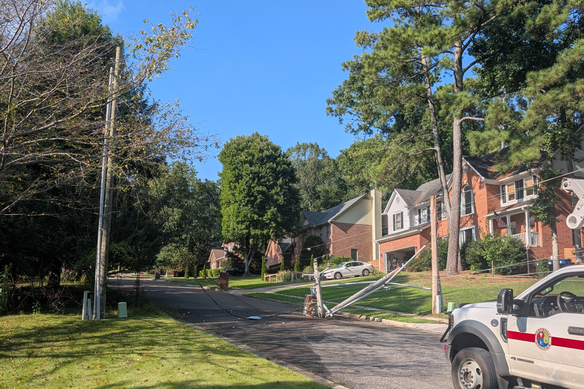
Figure 1. The pole at the right broke at mid height. The standing stub carries a fresh, light colored fracture surface against a weathered grey exterior, and the upper section is lying in the yard with the conductors. The bare pole at the left, across the street, lost its top when the conductors were pulled away from it. Author photograph.
The poles in this neighborhood are old. Most of them are silvered grey, deeply checked along their length, and hard and brittle to the knuckle. That is a familiar sight across north Alabama and across most of the country, and it raises a question worth working through with numbers rather than adjectives: how much strength does a weathered pole actually lose, and why does one fail on a still morning two days after the wind that hurt it?
A note before anything technical. Never approach a downed line, and never assume a conductor lying in the grass is dead. Poles that are still standing after a wind event can be carrying a fraction of their original strength with no external sign of it. Report and stay back.
What a Distribution Pole Is Designed to Carry
A wood distribution pole is a tapered cantilever fixed in soil. It is graded to ANSI O5.1, which assigns a class by the horizontal load the pole must resist when that load is applied two feet below the tip, with the pole embedded to the usual depth of ten percent of its length plus two feet. Southern Yellow Pine and Douglas Fir are both assigned a designated fiber stress of 8,000 psi. The class determines the required tip circumference and, through the fiber stress, the required circumference at the groundline.
| Class | Horizontal class load, lb | Minimum tip circumference, in | Typical use |
|---|---|---|---|
| 1 | 4,500 | 27 | Heavy angle, transmission underbuild |
| 2 | 3,700 | 25 | Corners, dead ends |
| 3 | 3,000 | 23 | Heavier tangent runs |
| 4 | 2,400 | 21 | The ordinary residential tangent pole |
| 5 | 1,900 | 19 | Light service, secondary only |
Table 1. ANSI O5.1 pole classes. The class load is applied two feet below the tip.
Take the pole in the photograph as a 40 ft Class 4 Southern Pine pole, which is the most common residential tangent pole in the country. Embedment is 6 ft, so 34 ft stands above grade and the class load acts 32 ft above the groundline. The required moment capacity at the groundline is
$$M_{cap} = 2400 \times 32 \times 12 = 921{,}600 \text{ in-lb}$$
and the required section modulus follows from the designated fiber stress,
$$S = \frac{M_{cap}}{F_b} = \frac{921{,}600}{8000} = 115.2 \text{ in}^3, \qquad S = \frac{\pi d^3}{32}$$
which gives a groundline diameter of 10.55 in, or a circumference of about 33 in. That agrees with the ANSI table to within half an inch, which is a useful check that the class system is nothing more mysterious than a round cantilever sized for a bending stress.
Everything about a wood pole follows from the cube in that expression. Strength scales as $d^3$ and stiffness as $d^4$, so wood lost near the surface, where the moment arm is longest, is expensive, and wood lost at the center is nearly free. That single fact explains most of what follows.
How Much Wind Does It Take?
The demand side is straightforward. Velocity pressure in customary units is
$$q = 0.00256\,V^2$$
with $q$ in psf and $V$ in mph. The pole itself presents a tapered projected area of roughly 24 sq ft above grade, with a drag coefficient near 0.9 for a rough round section. The conductors present much more area at a much longer lever arm: three primary phases and a neutral at 28 to 32 ft, plus a communications bundle lower down, each carrying half of the two adjacent spans. For 150 ft spans, that is the dominant term.
Running the sum for a range of gust speeds gives Figure 2. A gust of 70 mph produces a groundline moment of about 246,000 in-lb. That is 27 percent of the capacity of a new Class 4 pole. A sound pole of this class, in this configuration, does not fail until roughly 135 mph.
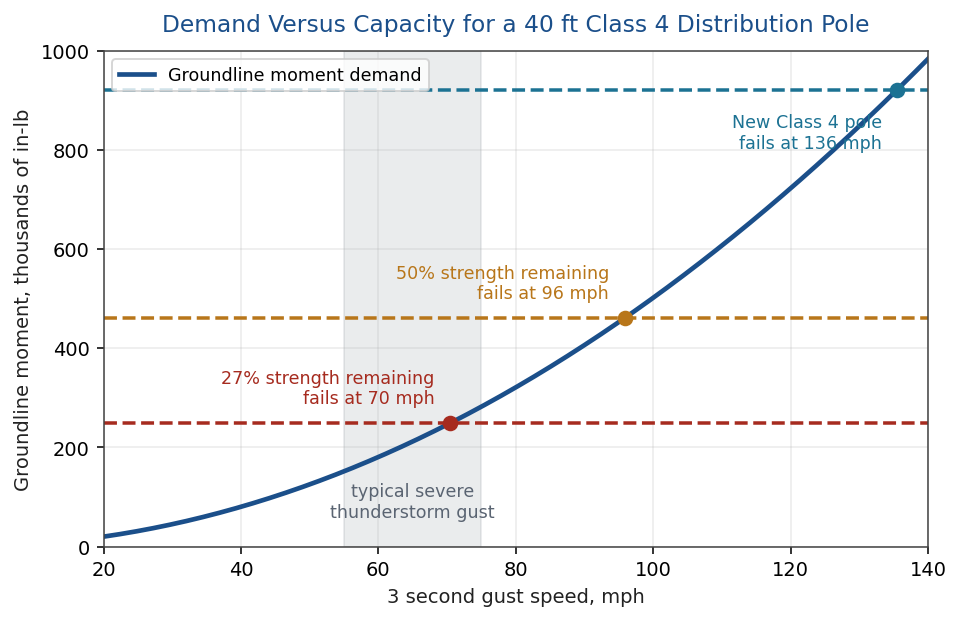
Figure 2. Demand grows with the square of gust speed. A new pole has a very large margin against an ordinary thunderstorm. A degraded pole does not.
This is the number that frames the whole problem. A neighborhood pole that comes down in a summer thunderstorm has almost always lost the large majority of its original strength before the storm arrives. The wind is the trigger. The loss of section is the cause.
Where a Tapered Pole Breaks, and Where This One Did
The pole in the photograph did not break at the groundline. It broke through at mid height, and that single observation carries more diagnostic information than anything else in the picture.
Both demand and capacity fall as you move up a pole. Demand falls because there is less load above the section and the lever arms shorten. Capacity falls because the pole tapers and section modulus goes as the cube of the diameter. Which one falls faster decides where the pole breaks. For a single load $P$ at the tip of a pole tapering linearly from $d_g$ at grade to $d_t$ at the top, write $d(z) = d_g(1{-}kz)$ with $k = (1{-}d_t/d_g)/H$. Then
$$\sigma(z) = \frac{32P(H{-}z)}{\pi d_g^3 (1{-}kz)^3}$$
and setting the derivative to zero gives a stress maximum at
$$z_{max} = \frac{3H}{2} {-} \frac{1}{2k}$$
For these dimensions $k$ is 0.0108 per ft and $z_{max}$ lands about 4.7 ft above grade, not at the base. Adding the distributed wind on the pole itself pulls the maximum back down to the groundline, but only just.
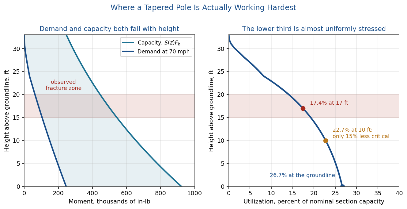
Figure 3. Demand and capacity fall together, so the utilization profile is remarkably flat over the lower third of the pole.
That flatness is the first result worth having. A tapered pole is not a structure with one critical section. Utilization runs 26.7 percent of nominal at grade, 22.7 percent at 10 ft, and is still 17.4 percent at 17 ft. A defect 10 ft up only has to make that section 15 percent weaker than the groundline wood in order to control the failure. The pole is close to being a constant-stress member by accident, which is elegant and also unforgiving, because it means there is no single place to inspect.
The second result is the diagnostic one. A sound pole loaded by wind breaks at or very near the groundline, because that is where utilization peaks. This pole did not. For the fracture to occur at roughly 17 ft while the groundline, working at 1.5 times the utilization, survived, the wood at the fracture must have been locally much weaker than the wood below it. In absolute terms, at a 70 mph gust, that section retained something on the order of 17 percent of its nominal capacity.
Break elevation is therefore evidence, and it points away from the usual suspect. Groundline decay produces groundline breaks. A break well up the pole points to a local defect at that specific section, and the list is short:
- Woodpecker cavities. Pileated excavations in the southeast are typically 10 to 25 ft up, run several inches across, and remove wood from one face, which is the worst possible geometry for bending.
- Lightning damage. A strike can drive a longitudinal split or separate the outer shell, and it usually leaves the lower pole intact.
- Old hardware. Through bolt holes, abandoned framing, and holes drilled for street lights or risers leave both a reduced section and a water path into untreated heartwood, well above the treated groundline zone.
- Top rot working downward from an unsealed or badly checked top.
- A large knot or a run of spiral grain, which is a local strength reduction that the grading rules tolerate within limits.
Any of these creates a strength discontinuity, and on a utilization curve as flat as the one in Figure 3, it takes very little discontinuity to move the failure a long way up the pole.
Read the fracture before the crew hauls it off. A long, feathered break with fibers pulled out over many inches is a tension failure in tough, sound wood. A short, blunt, squared-off break with a granular face is a brash failure, characteristic of wood that has lost toughness to age or decay. The break in Figure 1 looks closer to the second than the first, which is consistent with how these poles feel to the knuckle, but that is a judgment made at fifty feet. The things to check up close are the length of the splinters, whether the wood at the break is discolored or punky, and whether there is a cavity or a bolt hole in the fracture plane.
There is one piece of good news in all of this. The portion below the break, including the groundline and the embedded length, carried the load right up to the failure. Whatever was wrong with this pole, a standard groundline inspection would very likely have passed it.
Why the Poles Look the Way They Do
A treated pole is not treated all the way through. Southern Pine takes preservative readily in the sapwood, which forms an outer shell perhaps one to two inches deep, but the heartwood at the center accepts very little. The pole is therefore a treated tube around an untreated core. As long as the tube is continuous, decay fungi cannot reach the core, because they need free moisture, oxygen, and untreated cellulose all at once.
Checks break that logic. A check is a radial split that opens as the pole dries and as it cycles through wet and dry seasons. Checks run parallel to the grain, they are not fatigue cracks in the metallurgical sense, and by themselves they are considered normal. The problem is that a check deeper than the treated shell is a chimney into the untreated core. Rain runs down the pole, enters the check, and stops at the groundline where the wood stays damp and the oxygen is still plentiful. That is why internal decay in a wood pole is nearly always found in the zone from about 18 in below grade to about 24 in above it, and why the surface of a badly decayed pole can look perfectly sound.
The same three requirements have to be met wherever decay occurs, and above grade they are met anywhere something holds water against untreated wood. A deep check that catches rain, a bolt hole, a woodpecker cavity, an unsealed top: each is a small groundline zone hoisted twenty feet into the air, and each is invisible from the ground.
The grey, brittle feel of a weathered pole is a separate effect, and a shallower one. Ultraviolet exposure degrades lignin in the outer millimeter or so, and the resulting surface erosion, checking, and loss of resilience are real but structurally minor. What matters is what is happening a few inches in, and at the groundline, where nobody looks.
What Decay and Checks Actually Cost
Three damage patterns matter, and they are not equally serious.
Internal decay leaving a sound shell. For an annulus of outside diameter $d_o$ and inside cavity $d_i$,
$$S = \frac{\pi (d_o^4 {-} d_i^4)}{32\,d_o}$$
A 2 in shell on a 10.55 in pole retains 85 percent of the original section modulus. A 1 in shell still retains 57 percent. This is why utility maintenance criteria are written in terms of remaining shell thickness, and why a pole a lineman can hear ringing hollow may still be perfectly serviceable. Material near the neutral axis was never doing much work.
A one-sided pocket. Decay that eats in from one face is far worse than the same volume removed from the center, because it moves the neutral axis and removes the extreme fiber. Losing 3 in from one side of a 10.55 in pole leaves only 55 percent of the section modulus about the tension face. The same 3 in taken as a symmetric internal cavity would cost almost nothing.
A through check. This is the one that surprises people. A split that runs the full depth of the section, on the plane of bending, destroys longitudinal shear transfer between the two halves. Each half then bends about its own centroid. For a semicircle of radius $R$, the moment of inertia about its own centroidal axis is
$$I_{half} = \left(\frac{\pi}{8} {-} \frac{8}{9\pi}\right) R^4 = 0.1098\,R^4$$
Summing two halves and dividing by the distance to the extreme fiber gives a section modulus ratio of 0.486 against the intact round, and a stiffness ratio of only 0.279. A single full-depth check can therefore cost half the bending strength and nearly three quarters of the stiffness about the worst axis, while the pole looks entirely normal from ten feet away.
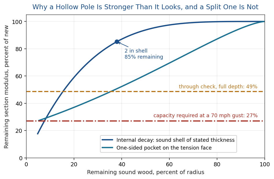
Figure 4. Where the wood goes matters more than how much of it goes.
No single one of these defects gets a section down to the 17 percent that the fracture elevation requires at a 70 mph gust. Stacked, they very nearly do. The table below applies the same ratios at the 8.62 in diameter that a 40 ft Class 4 pole has at 17 ft. Treating the ratios as multiplicative is rough, since the defects are not independent, but it shows the trend:
| Condition at the fracture section, 17 ft up | Ratio | Cumulative remaining strength |
|---|---|---|
| Sound section, 8.62 in diameter | 1.00 | 100% |
| Internal decay to a 2 in sound shell | 0.92 | 92% |
| Full-depth check on the plane of bending | 0.49 | 45% |
| Woodpecker cavity or bolt hole, 3 in into one face | 0.45 | 20% |
Table 2. Three ordinary defects, none of them individually alarming, arriving within a few points of the 17 percent that this failure required.
Why It Failed Two Days After the Storm
This is the part that is genuinely interesting from a structural dynamics standpoint, because the pole did not fail during the peak load. It failed under a load it had already survived.
Wood is one of the few structural materials whose strength depends strongly on how long the load is applied. The classical description is the Madison curve, developed at the Forest Products Laboratory,
$$SL = 18.3 + 108.4\,t^{-0.04635}$$
where $SL$ is the load level as a percentage of the strength measured in a standard five minute ramp test, and $t$ is the time to failure in seconds. The curve is calibrated so that $SL$ is essentially 100 percent at five minutes. A load carried for one second can be 127 percent of that value. A load carried for two days can only be 80 percent. A load carried for ten years can only be 62 percent.
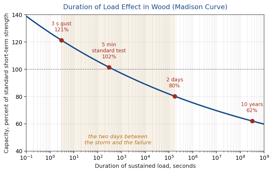
Figure 5. Wood strength as a function of load duration. The gust and the two-day wait sit on opposite ends of a factor of 1.5.
The ratio between the three second gust value and the two day value is 121 over 80, or 1.5. A pole that survives a gust at the very limit of its short-term capacity is therefore not safe at that same load an hour later, let alone two days later. Creep rupture in wood is a slow crack growth process in the cell wall, and it does not care that the wind has stopped.
Three things plausibly conspired here, and they reinforce one another:
Damage during the storm. Partial fiber rupture on the tension face at the weak section leaves no external mark, and nobody is looking twenty feet up in any case. The pole came out of the storm weaker than it went in, and nothing about its appearance would say so.
Sustained load afterwards. A pole left out of plumb carries an eccentric gravity moment it did not have before, and any residual unbalance in conductor tension from a neighboring span stays applied indefinitely. That load then sits on the far end of the Madison curve.
A loosened socket in wet soil. Storm loading works the pole back and forth against the soil and opens a gap at the surface, and the rain saturates the backfill. Reduced rotational restraint lowers the effective point of fixity and softens the pole. The direct moment increase is largest near grade, so it is not the whole story for a break at mid height, but the added lean and the larger sway both raise the second-order moment along the entire length. The pole is quietly getting worse for days.
Delayed failures after storms are common enough that utilities treat post-event patrol as a distinct activity from outage restoration. The poles that come down on the day are the obvious problem. The ones that come down later are the reason for the patrol.
The Second Pole: A Load Path Problem, Not a Strength Problem
The pole across the street broke near its top. That is a completely different failure, and it should not be read as evidence that the second pole was also rotten.
A tangent pole carries almost no net longitudinal load in normal service. The conductor tension in the span on one side is balanced by the tension in the span on the other side, and the pole only has to resist the small difference plus transverse wind. This is why tangent poles are unguyed and why their tops are slender. When the first pole goes down, that balance is destroyed. The far span keeps pulling and the near span no longer pushes back, so the surviving pole sees the full residual tension applied longitudinally, right at the crossarm.
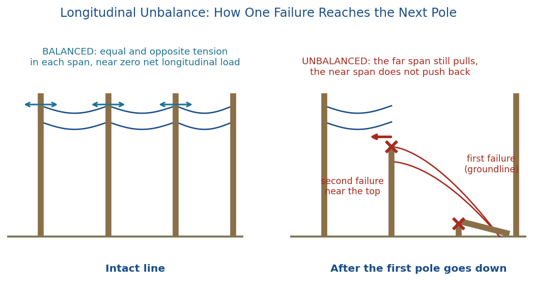
Figure 6. The mechanism by which a single pole failure becomes a two pole failure.
Run the numbers at the top of the pole. Four feet below the tip the diameter is about 7.1 in, giving a section modulus of 35.7 in3 and a moment capacity of 285,000 in-lb even at the full 8,000 psi. With the conductors attached one foot below the tip, the lever arm is three feet, so a new pole tolerates about 7,900 lb of longitudinal pull at that location.
Now the demand. Three primary phases at roughly 1,200 lb each, a neutral, and a communications messenger give something on the order of 6,000 lb of residual unbalanced tension. Applied statically that is under the capacity. Applied as a step, it is not.
The Dynamics of the Release
The surviving pole is a cantilever with a tip mass. For the 34 ft Class 4 geometry, with a modulus near 1.4 million psi, an effective moment of inertia of about 335 in4 after accounting for taper, a pole weight near 620 lb and perhaps 300 lb of hardware and tributary conductor at the top,
$$k = \frac{3EI}{L^3} \approx 21 \text{ lb/in}, \qquad f_n = \frac{1}{2\pi}\sqrt{\frac{k}{m_e}} \approx 0.67 \text{ Hz}$$
so the natural period is about 1.5 sec. The tension release, on the other hand, is fast. A longitudinal disturbance travels along a steel messenger at roughly 5,000 m/sec, crossing a 150 ft span in about 9 msec. Even allowing for slack take-up and the slower transverse wave, which for a 1,200 lb tension and 0.69 kg/m mass runs at only about 88 m/sec, the load change is complete in a small fraction of the pole period.
A load applied in much less than one natural period is a step, and an undamped step gives a dynamic amplification factor of 2. Figure 7 shows the response for three release times against a 1.5 sec period with 2 percent damping.
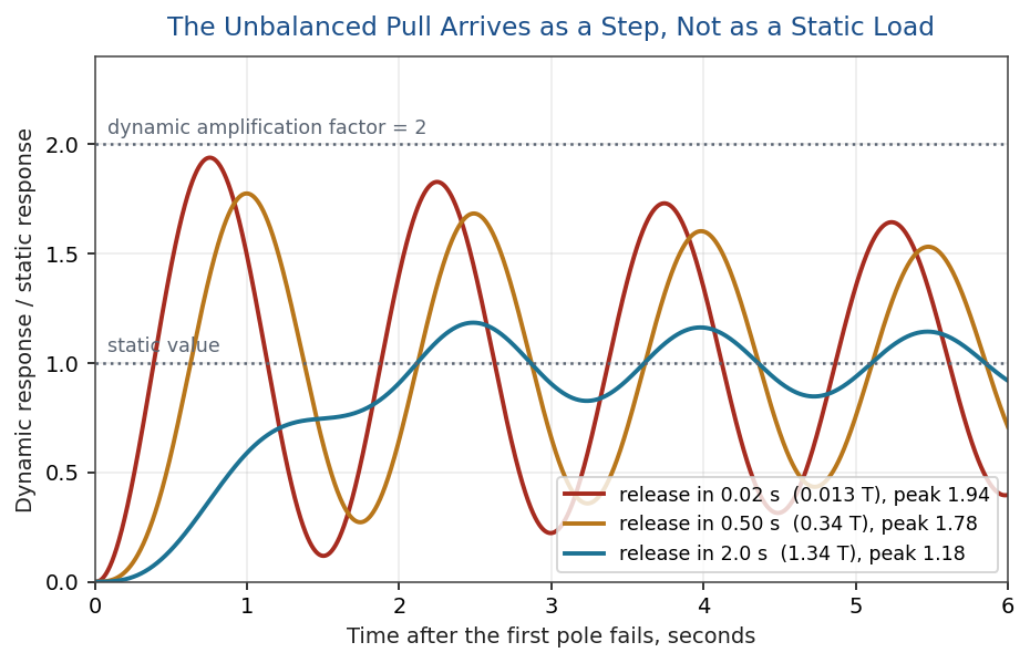
Figure 7. Rise time relative to the natural period governs the amplification. A fast release nearly doubles the load.
At a factor near 2, the effective demand at the top of the second pole is on the order of 12,000 lb against a new-pole capacity of about 7,900 lb. The second pole did not need to be defective. The dynamics alone were sufficient, and the duration of load effect works the other way here, since a load of a few tenths of a second can be carried at about 125 percent of the standard strength, which is nowhere near enough to close a gap of that size.
There is a second dynamic effect worth naming, because it is the same one that governs shock severity in every other structure. When the falling pole jerks a cable, the stress in that cable follows from the particle velocity, not from any static calculation:
$$\sigma = \rho c V$$
For steel, $\rho c$ is about 39 MPa per m/sec. A cable end yanked at 3 m/sec sees a transient of roughly 118 MPa, or 17 ksi, superimposed on whatever tension it already carried, and it sees it within milliseconds. This is the same stress-velocity relationship that governs shock response spectra severity, and it is why the snap loads in a cascading line failure are so much larger than the static tensions suggest.
The distinction worth carrying away. The first pole failed because it was degraded. The second pole failed because of the system it was part of. Cascading line failures are not evidence that every pole in the run was rotten, and treating them that way misdirects the inspection program.
What Inspection Actually Finds
Given that the critical damage is internal and below grade, visual inspection from a truck is nearly worthless for the failure mode that matters. The standard methods, in rough order of intrusiveness:
| Method | What it detects | Limitation |
|---|---|---|
| Visual, from the ground | Lean, checks, woodpecker holes, hardware | Blind to the groundline zone |
| Hammer sounding | Large internal voids, by change in ring | Subjective, misses shell rot and early decay |
| Prod and excavate to 18 in | External decay below grade | Labor, and it breaches the backfill |
| Increment boring | Shell thickness directly | Samples one line only, leaves a hole to plug |
| Resistance drilling | Density profile across the full diameter | One diameter per pass, interpretation required |
| Sonic or ultrasonic tomography | Two dimensional map of the section | Slower, more equipment, more cost per pole |
Table 3. Inspection methods and what each one can and cannot see.
Remedial options are correspondingly graded. Groundline treatment with a preservative bandage arrests decay in a pole that still has adequate shell. A steel or fiberglass truss bolted across the groundline restores capacity to a pole that does not. Replacement is the answer when the remaining strength falls below the threshold the utility uses, commonly two thirds of the original value. Storm guying, or converting selected structures to a heavier class at intervals along a long tangent run, is the direct countermeasure for the cascade mechanism, since a guyed pole every so often stops the unbalanced pull from propagating down the whole line.
Closing
A wooden utility pole is a cantilever with a strength that decays with time in three separate senses. Decay in the biological sense removes section where it matters most. Duration of load removes capacity as a function of how long the load stays on. And the system around it removes the balanced boundary condition it was designed to have, the moment a neighbor fails.
The poles on our street have been standing in Alabama humidity for decades. They look weathered because they are, but the greying and the surface checks are the visible fraction of a problem that is mostly hidden, either a few inches below the grass or fifteen feet above it. This one chose the second. The interesting engineering question is not why it snapped in the wind. It is why the rest did not.
Note on assumptions: the class, span, tension and material values used above are representative of typical residential distribution construction and are not measurements from these particular poles. The conclusions are about the mechanisms, not about the specific structures in the photograph.
Related free ebooks on shock, vibration and stress-velocity are available at Tom’s Ebooks.