Nearly every random vibration fatigue course teaches that the response of a single-degree-of-freedom system to broadband base excitation has Rayleigh-distributed peaks. The claim is repeated so often that it has hardened into doctrine. It is a good approximation for the largest peaks, which is why it has survived. But it is quantitatively wrong for the small peaks, and the error is not small. This post measures the discrepancy, shows why Dirlik’s one-exponential-plus-two-Rayleigh form captures it, and then asks the question that actually matters: does it change the answer? For classical S-N fatigue on a single mode the honest answer is barely — but that reprieve disappears the moment a second mode participates. For fracture mechanics crack growth the honest answer is more complicated, and more interesting, than the usual telling. And for crack formation, which is a different calculation run by a different code on the same spectrum file, the answer inverts again.
The last third of this post is devoted to that last point, because it is where the most expensive misunderstandings live. NASGRO is not one program. NASFLA computes damage tolerance crack growth life. NASFORM computes crack formation life by stress-life or strain-life. Handed the same load block and the same structure, the two modules can return answers separated by four or five orders of magnitude — and in most cases that is not a bug in either code. It is a consequence of the exponent each one applies to the amplitude distribution, and of the fact that the stress the two of them want is not the same stress.
Where the Rayleigh Assumption Comes From
Consider a stationary Gaussian random process with zero mean and standard deviation $\sigma$. If the process is ideally narrowband — energy concentrated in a vanishingly thin band around a single frequency — then the time history looks like a sine wave with a slowly varying envelope. Every zero upcrossing is followed by exactly one maximum, and the amplitude of that maximum equals the envelope value. The envelope of a narrowband Gaussian process is Rayleigh distributed, and therefore so are the peaks:
$$p(\eta) \; = \; \eta \, e^{-\eta^2/2}, \qquad \eta = \frac{A}{\sigma}, \qquad \eta \ge 0$$
This gives the familiar reference values that show up in every peak-statistics report: the mean absolute peak is $\sqrt{\pi/2}\,\sigma = 1.2533\,\sigma$, and the RMS peak is $\sqrt{2}\,\sigma = 1.4142\,\sigma$. When a measured or synthesized time history returns a mean-to-sigma ratio noticeably below 1.2533, that is the first clue that the narrowband idealization has broken down.
The logic is sound. The problem is the premise. A lightly damped SDOF driven by broadband base input is not ideally narrowband, and the departure is larger than most engineers expect.
The Exact Result: Rice, Not Rayleigh
For any stationary Gaussian process, the distribution of maxima is known exactly. It was derived by S. O. Rice in 1945 and it depends on a single bandwidth parameter. Define the spectral moments of the one-sided response power spectral density $G(f)$:
$$m_n \; = \; \int_0^\infty f^{\,n} \, G(f) \, df$$
The rate of mean-level upcrossings, the rate of maxima, and the irregularity factor are then
$$n_0 = \sqrt{\frac{m_2}{m_0}}, \qquad E[P] = \sqrt{\frac{m_4}{m_2}}, \qquad \gamma = \frac{n_0}{E[P]} = \frac{m_2}{\sqrt{m_0 \, m_4}}$$
The irregularity factor $\gamma$ is the fraction of maxima that are also upcrossings. It runs from 0 for broadband white noise to 1 for an ideal narrowband process. Rice’s distribution of maxima is a weighted sum of a Gaussian term and a Rayleigh term:
$$p(\eta) \; = \; \frac{\sqrt{1-\gamma^2}}{\sqrt{2\pi}} \, \exp\!\left[ \frac{-\eta^2}{2(1-\gamma^2)} \right] \; + \; \gamma \, \eta \, e^{-\eta^2/2} \, \Phi\!\left( \frac{\gamma \eta}{\sqrt{1-\gamma^2}} \right)$$
where $\Phi$ is the standard normal cumulative distribution function. Setting $\gamma = 1$ kills the Gaussian term and recovers Rayleigh exactly. Setting $\gamma = 0$ leaves a pure Gaussian, which is correct for white noise where maxima occur everywhere including well below the mean. So the Rayleigh model is not merely an approximation — it is the $\gamma = 1$ endpoint of a one-parameter family, and the whole question is how far the real system sits from that endpoint.
The critical distinction. The Gaussian term in the Rice distribution has support on the negative axis. A finite fraction of the maxima of a real SDOF response lie below zero — they are local maxima on the downslope of a larger oscillation. The Rayleigh model assigns those events zero probability. They are not rare. They are not a rounding error. In the example below they account for roughly one maximum in ten.
Why a Real SDOF Is Never Narrowband
The relative displacement of a base-excited SDOF, which is the quantity proportional to spring stress, has the frequency response function
$$\frac{Z(\omega)}{\ddot{Y}(\omega)} \; = \; \frac{-1}{\left( \omega_n^2 – \omega^2 \right) + j \, 2 \zeta \omega_n \omega}$$
At frequencies well above resonance this rolls off as $1/\omega^2$, so the response PSD rolls off as $f^{-4}$. Now look at the fourth spectral moment. Its integrand is $f^4 G(f)$, which above resonance behaves as $f^4 \cdot f^{-4} = \text{constant}$. The integral does not converge. As the upper band limit of the base input is pushed higher, $m_4$ grows without bound, $E[P]$ grows without bound, and $\gamma$ marches toward zero.
This is not an academic curiosity. It means the number of peaks in an SDOF response is not a property of the SDOF at all — it is set by the bandwidth of the input. Two analysts using the same natural frequency and the same Q, but specifying the base input to 2000 Hz versus 10000 Hz, will count very different numbers of maxima and will get very different irregularity factors from the same physical structure.
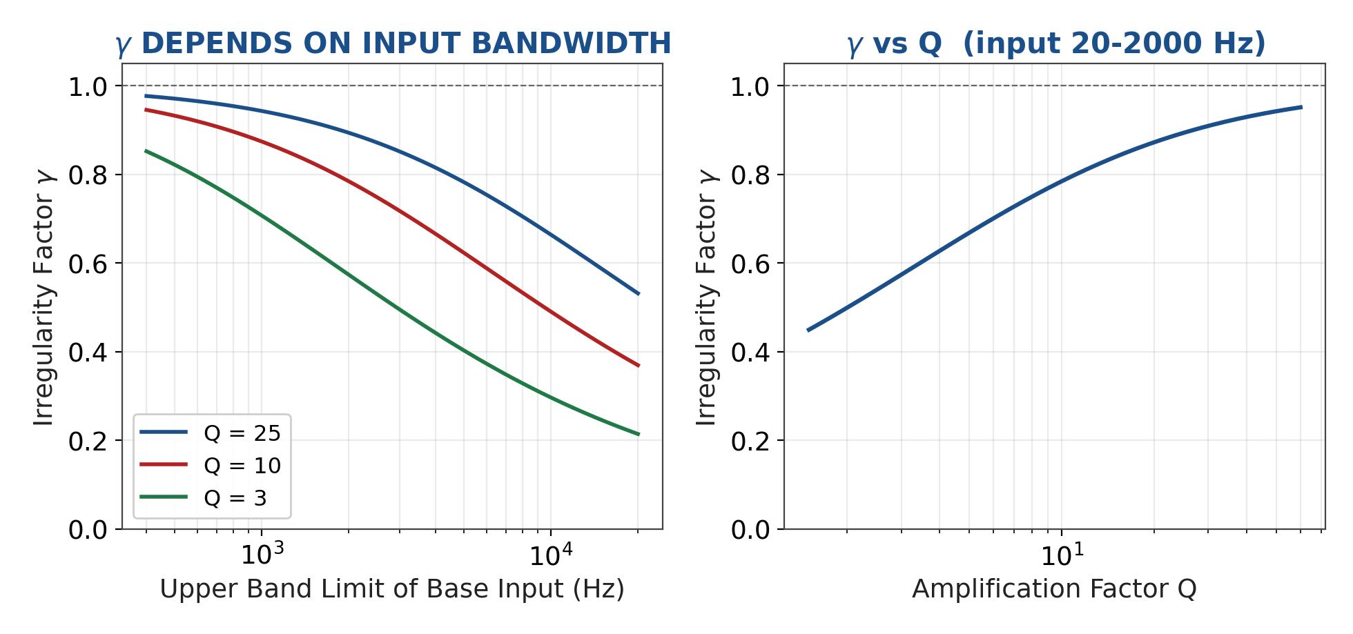
The left panel makes the point. For Q = 10 and an input band limit of 500 Hz, the irregularity factor is 0.93 and the Rayleigh assumption is defensible. Extend the same input to 20000 Hz and $\gamma$ falls to 0.37. The right panel shows the Q dependence at a fixed 20 to 2000 Hz input band: even at Q = 60, $\gamma$ only reaches about 0.9. The narrowband ideal is approached slowly and never arrived at.
For absolute acceleration response the situation is worse still. That transfer function rolls off only as $1/\omega$, so the response PSD rolls off as $f^{-2}$ and even $m_2$ fails to converge. The upcrossing rate itself becomes unbounded. Whenever peak statistics are computed on an absolute acceleration signal rather than on a stress-proportional relative displacement, the numbers carry an additional bandwidth artifact on top of everything discussed here.
A Numerical Experiment
The remainder of this post uses a single controlled case. The base input is band-limited Gaussian white noise, flat at 0.10 G²/Hz from 20 to 2000 Hz, for an overall level of 14.07 GRMS. The SDOF has a 200 Hz natural frequency. The primary case is Q = 10, with Q = 25 and Q = 3 carried along for contrast. The record is 900 seconds at 8192 samples per second, and the response quantity is relative displacement. Peaks were extracted with no hysteresis gate, and cycles were counted with a self-contained ASTM E1049 three-point rainflow algorithm with the residual stack counted as half cycles.
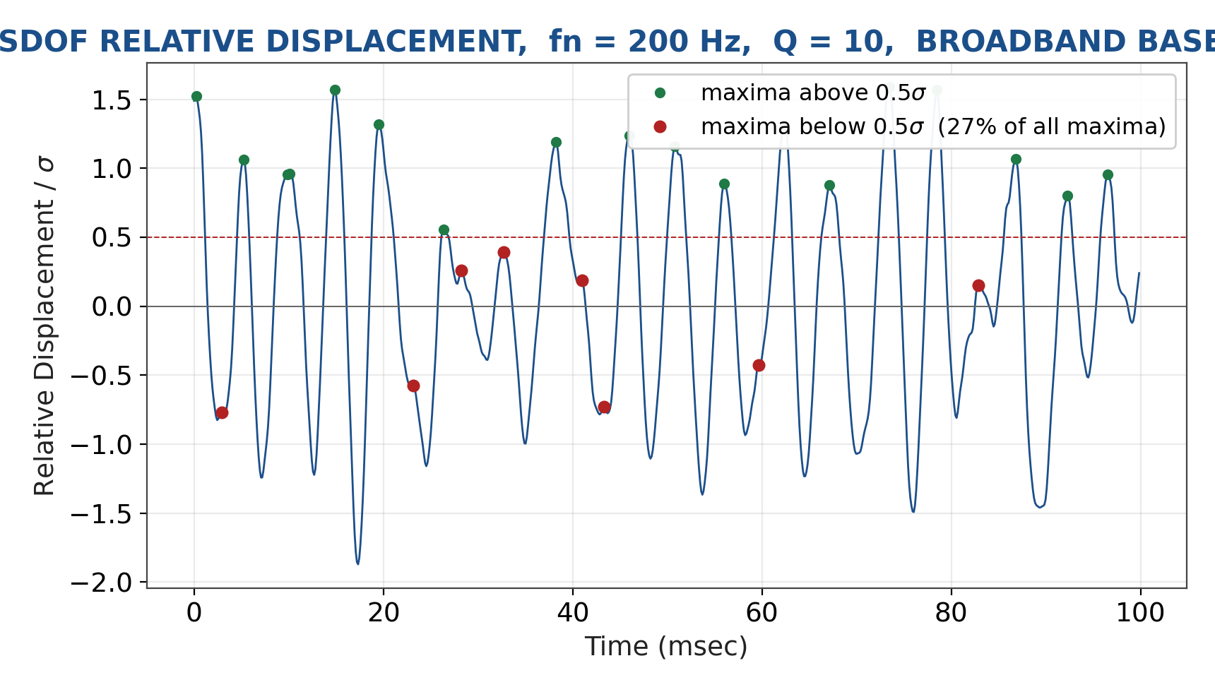
One hundred milliseconds of the Q = 10 response is shown above, with maxima marked. The large oscillation at 200 Hz is the resonant response everyone expects. Riding on it are the small maxima marked in red — the direct, non-resonant transmission of the broadband input through the same structure. These are the low peaks. They are perfectly real, they are counted by any peak-picking or rainflow routine, and the Rayleigh model says they do not exist.
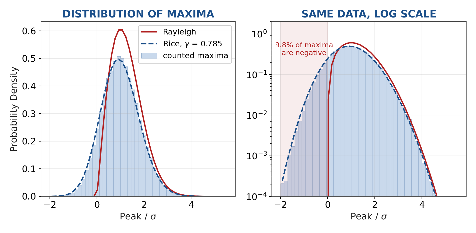
The measured distribution of maxima is compared with both models above. Rayleigh fails badly below about $1.5\sigma$ and is respectable above $2.5\sigma$. The Rice distribution, using the irregularity factor computed from the spectral moments with no fitting whatsoever, tracks the data across the full range including the negative-peak population highlighted in the log-scale panel. Note that a negative peak value in the Rice curve means: a local high point that happened while the signal was still below zero.
| Peak Statistic | Rayleigh | Q = 25 | Q = 10 | Q = 3 |
|---|---|---|---|---|
| Irregularity factor $\gamma$ | 1.000 | 0.894 | 0.785 | 0.574 |
| Maxima per second | 200.0 | 220.8 | 248.8 | 334.3 |
| Mean absolute peak / $\sigma$ | 1.2533 | 1.1563 | 1.0731 | 0.9446 |
| RMS peak / $\sigma$ | 1.4142 | 1.3477 | 1.2816 | 1.1641 |
| Fraction of maxima below zero | 0.0 | 0.047 | 0.098 | 0.202 |
| Fraction of maxima below $0.5\sigma$ | 0.118 | 0.195 | 0.268 | 0.394 |
| Largest peak / $\sigma$ | — | 4.80 | 4.83 | 5.00 |
Note the mean absolute peak column. Even at Q = 25, an unusually lightly damped structure, the ratio is 1.156 rather than 1.2533. At Q = 10 it is 1.073, a 14 percent shortfall. Field data is typically further off still, because real structures are multi-modal and real inputs are not flat. Measured aerospace buffet response records routinely return mean-to-sigma ratios in the 0.81 to 0.86 range, corresponding to irregularity factors far below anything an SDOF idealization would suggest.
From Peaks to Cycles: Dirlik’s Formula
A point worth making explicitly, because it is a frequent source of confusion: the Rice distribution describes peaks, while Dirlik’s formula describes rainflow ranges. They are different quantities answering different questions, but both exist for the same reason — the low-amplitude population that the narrowband ideal ignores.
Rainflow counting pairs maxima with minima according to the hysteresis-loop closure rules, so the resulting cycle set is not simply the peak set. Dirlik obtained an empirical closed-form expression for the rainflow range distribution by regression against a large set of Monte Carlo simulations. In terms of the normalized range $Z = S / (2\sqrt{m_0})$, which is simply amplitude divided by $\sigma$:
$$p(Z) \; = \; \frac{D_1}{\bar{Q}} e^{-Z/\bar{Q}} \; + \; \frac{D_2 \, Z}{R^2} e^{-Z^2/(2R^2)} \; + \; D_3 \, Z \, e^{-Z^2/2}$$
with coefficients determined entirely by the first four spectral moments:
$$x_m = \frac{m_1}{m_0}\sqrt{\frac{m_2}{m_4}}, \quad D_1 = \frac{2\left(x_m – \gamma^2\right)}{1+\gamma^2}, \quad R = \frac{\gamma – x_m – D_1^2}{1 – \gamma – D_1 + D_1^2}$$
$$D_2 = \frac{1 – \gamma – D_1 + D_1^2}{1 – R}, \quad D_3 = 1 – D_1 – D_2, \quad \bar{Q} = \frac{1.25\left(\gamma – D_3 – D_2 R\right)}{D_1}$$
The structure is exactly the one exponential plus two Rayleigh terms of the usual description. The third term, with coefficient $D_3$, is the classical narrowband Rayleigh contribution. The exponential term supplies the low-amplitude population. The second term interpolates between them. For the Q = 10 case the coefficients come out as $\gamma = 0.7846$, $x_m = 0.7650$, $D_1 = 0.1849$, $D_2 = 0.0528$, $D_3 = 0.7623$, $R = -0.2253$, and $\bar{Q} = 0.2311$.
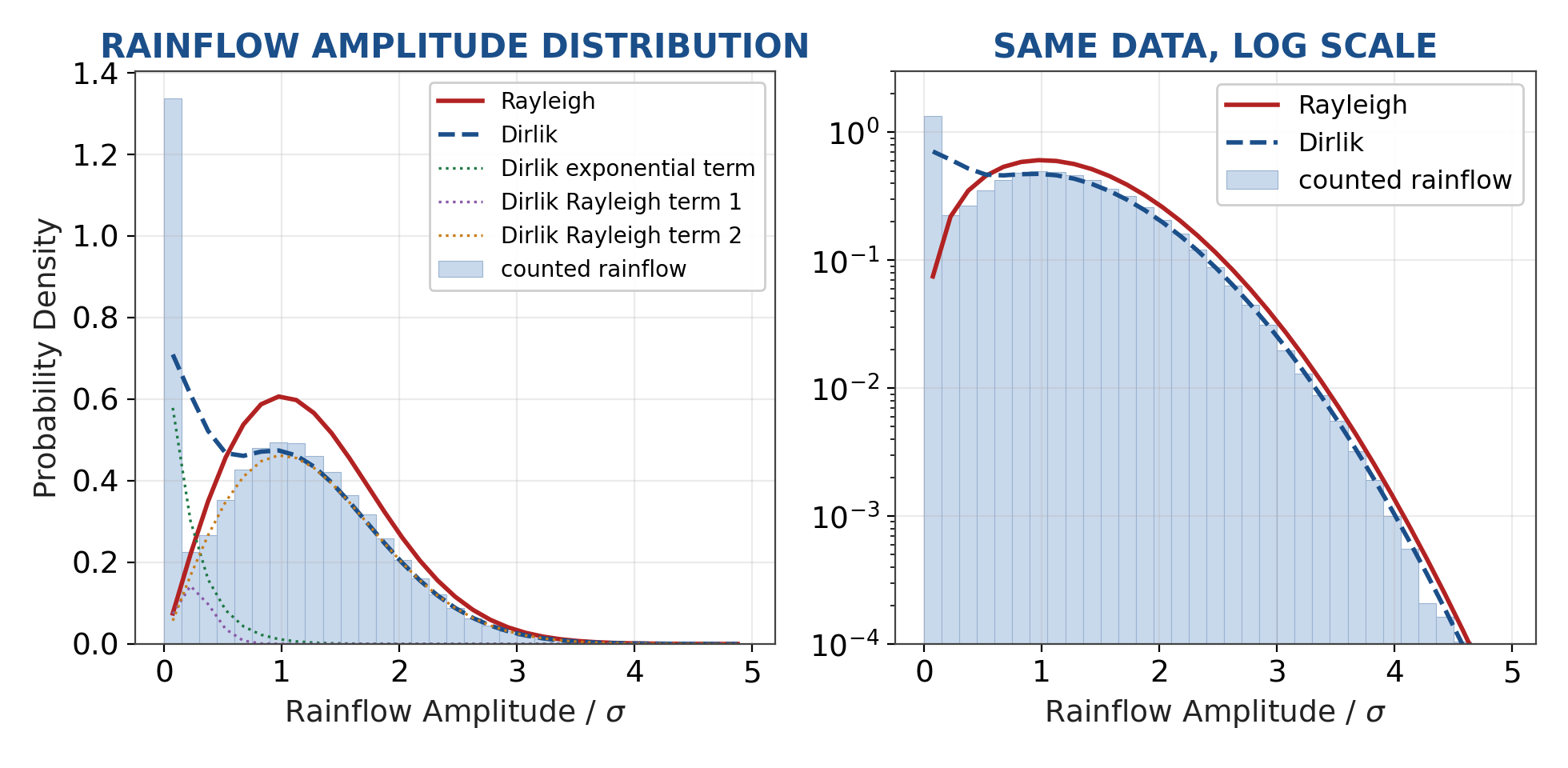
The individual Dirlik terms are drawn as dotted curves in the left panel. The Rayleigh model overshoots the counted data through the entire $0.5\sigma$ to $2\sigma$ region and undershoots below $0.4\sigma$. Dirlik follows the data closely across four decades of probability density.
A caution on the Dirlik coefficients. Note that $R$ came out negative for this case. The formula still evaluates, since only $R^2$ appears in the second term and $D_2$ is small here, but a negative $R$ signals that the input spectrum sits near the edge of the parameter space over which Dirlik performed his regression. Dirlik’s expression is an empirical fit, not a derivation, and it should be treated as such whenever the response spectrum is strongly bimodal or has an unusual bandwidth. This limitation is exactly what motivated the Meta-Dirlik correction method.
Effect on Classical Fatigue Damage
Here is where the story requires honesty rather than advocacy. Take the standard Palmgren-Miner accumulation with an S-N curve of slope $b$, so that relative damage is proportional to $\sum n_i S_i^{\,b}$. Compare three cycle sets over the same 900 second record: the counted rainflow, the Dirlik prediction, and the narrowband Rayleigh assumption of $n_0 T$ cycles with Rayleigh-distributed amplitudes.
| S-N Slope $b$ | Dirlik / Counted | Narrowband Rayleigh / Counted |
|---|---|---|
| 3.0 | 1.003 | 1.026 |
| 4.0 | 1.012 | 1.038 |
| 6.4 | 1.041 | 1.068 |
| 9.0 | 1.082 | 1.110 |
The narrowband Rayleigh assumption is conservative by 3 to 11 percent depending on slope. That is all. Against the factor-of-two and factor-of-three scatter inherent in S-N data, a 7 percent bias at $b = 6.4$ is not the thing that will sink a fatigue assessment.
The reason is the $S^{\,b}$ weighting. With $b$ in the range 6 to 9, damage is overwhelmingly controlled by the high-amplitude tail, and in that tail the two models agree closely. They must agree: the rate of crossings of a high level is governed by $n_0$, which both models share. The low peaks that Rayleigh gets wrong are precisely the cycles that a steep S-N exponent renders irrelevant. Two errors of opposite sign — Rayleigh predicts fewer total cycles but assigns them larger amplitudes — also partially cancel.
So if the only question is classical high-cycle fatigue with a steep S-N slope, the Rayleigh assumption survives. That is why it has survived.
Extension to Multi-Degree-of-Freedom Systems
Everything above generalizes to real hardware without modification, because the linear response of an MDOF system to Gaussian input is still Gaussian. The recipe is unchanged: recover the stress PSD at the critical location, integrate its first four spectral moments, and evaluate $\gamma$, the Rice distribution, and the Dirlik coefficients from those moments. No new theory is required. What changes is the answer, and it changes far more than the SDOF results would lead you to expect.
Consider two modes at 60 Hz and 400 Hz, each with Q = 15, combined at equal RMS contribution and driven by the same 20 to 2000 Hz base input. The table below adds a third mode at 1200 Hz, with a single 60 Hz mode carried as the reference case.
| Case, Q = 15 per mode | $\gamma$ | Mean abs peak / $\sigma$ | Std dev of cycle means | Rayleigh / counted, $b = 6.4$ | Dirlik / counted, $b = 6.4$ |
|---|---|---|---|---|---|
| Single mode, 60 Hz | 0.648 | 0.983 | $0.343\,\sigma$ | 1.002 | 0.967 |
| Two modes, 60 + 400 Hz | 0.651 | 0.976 | $0.599\,\sigma$ | 1.515 | 0.906 |
| Three modes, 60 + 400 + 1200 Hz | 0.609 | 0.937 | $0.647\,\sigma$ | 1.727 | 0.891 |
The first row is the important control. A single mode at 60 Hz has an irregularity factor of only 0.648, well below the narrowband ideal, yet the Rayleigh damage estimate is correct to within 0.2 percent. The cancellation described in the previous section is doing all the work: Rayleigh predicts too few cycles and assigns them amplitudes that are too large, and for a unimodal spectrum those errors offset almost exactly. Add a second mode and the cancellation collapses. The Rayleigh estimate becomes non-conservative by 52 percent, and by 73 percent with three modes, while Dirlik stays within roughly 10 percent. The mechanism is straightforward: the large stress cycles are produced at the rate of the lowest participating mode, near 60 Hz, but the narrowband model manufactures full-amplitude cycles at the mean upcrossing rate of the combined response, which is 285 Hz for the two-mode case. It counts nearly five times too many large cycles. Note also that $\gamma$ alone does not warn you — the single-mode and two-mode cases have essentially the same irregularity factor and completely different answers. Bandwidth is not the same as bimodality.
Two consequences follow for the crack growth discussion below. First, the small-riding-on-large geometry that produces the low peaks is dramatically amplified when a high-frequency mode rides on a low-frequency one, and with it the cycle-mean spread: the standard deviation of rainflow cycle means grows from $0.241\sigma$ for the earlier SDOF case to $0.599\sigma$ here, and the fraction of cycles with $R > 0$ rises from 18.5 to 33.7 percent. Second, a bimodal or widely separated modal response is precisely where Dirlik’s empirical regression is weakest, which is why the bimodal-specific spectral methods of Jiao and Moan, Fu and Cebon, Sakai and Okamura, Benasciutti and Tovo, and Zhao and Baker exist at all, and what the Meta-Dirlik correction is intended to address. For an MDOF assessment the practical instruction is short: never assume the peak distribution, recover the stress PSD at the critical element from the random response solution, and compute $\gamma$ and the modal participation before choosing a method.
Why Crack Growth Is a Different Problem
Fracture mechanics changes the weighting. The Paris law is
$$\frac{da}{dN} \; = \; C \left( \Delta K \right)^{n}, \qquad \Delta K = \Delta S \, Y \sqrt{\pi a}$$
with $n$ typically between 3 and 4 for aluminum alloys. In terms of stress range, growth per cycle scales as $\Delta S^{\,n}$ — equivalent to an S-N slope of about 3.2 rather than 6.4. Halving the exponent moves the center of gravity of the calculation dramatically toward the mid- and low-amplitude cycles.
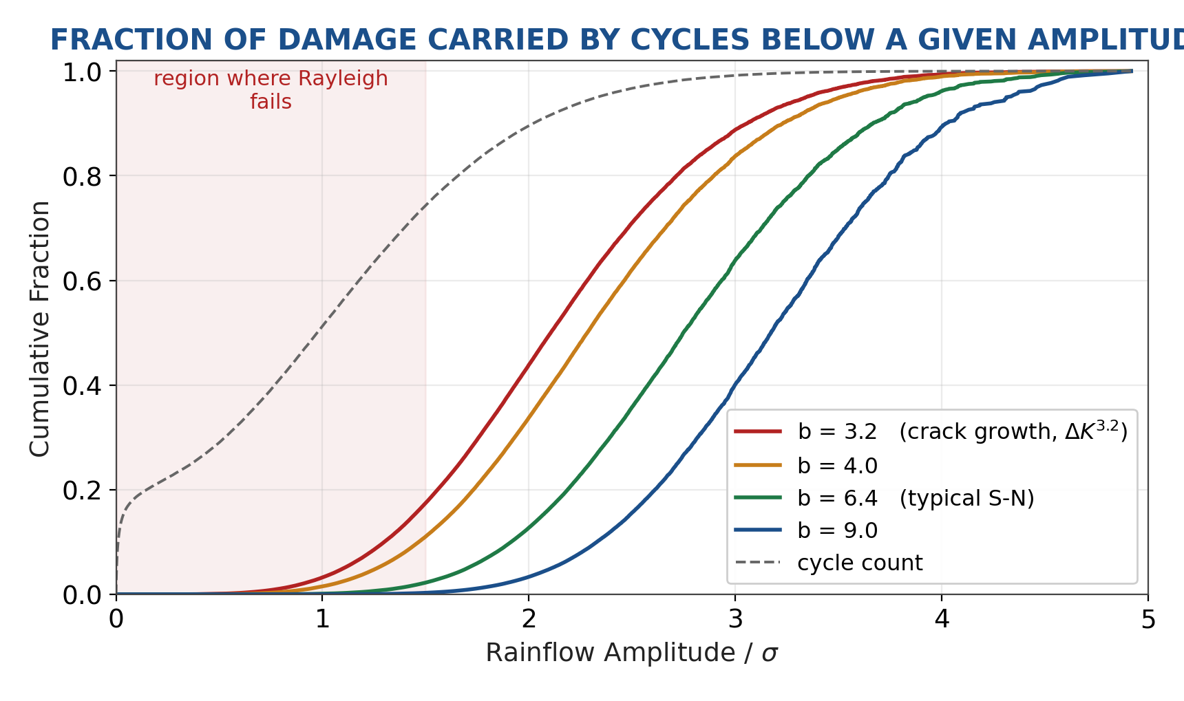
| Cycles with amplitude below | Fraction of cycle count | Fraction of $\Delta S^{3.2}$ (crack growth) | Fraction of $S^{6.4}$ (S-N) |
|---|---|---|---|
| $1.0\,\sigma$ | 0.513 | 0.032 | 0.001 |
| $1.5\,\sigma$ | 0.743 | 0.174 | 0.022 |
| $2.0\,\sigma$ | 0.896 | 0.438 | 0.127 |
| $2.5\,\sigma$ | 0.967 | 0.710 | 0.358 |
| $3.0\,\sigma$ | 0.992 | 0.888 | 0.638 |
Cycles below $2\sigma$ drive 44 percent of crack extension but only 13 percent of S-N damage. Below $1.5\sigma$ the split is 17 percent versus 2 percent. Crack growth draws roughly eight times as much of its driving from the amplitude band where the Rayleigh assumption is demonstrably wrong.
That said, a straight Paris integration with no threshold, run on all three cycle sets from the same 900 second record with identical initial and critical crack sizes, gives predicted lives within 3 percent of one another. The Rayleigh model returns 0.973 times the counted-rainflow life; Dirlik returns 0.997. The composition of the calculation is completely different, but the total comes out nearly the same, for the same cancellation reason as before.
The sensitivity appears once the model stops being a plain power law. Real crack growth analysis never is.
Three Mechanisms That Expose the Difference
1. The threshold is a moving amplitude filter. Below $\Delta K_{th}$ a cycle produces no growth at all. Since $\Delta K = \Delta S \, Y \sqrt{\pi a}$, the stress range required to reach threshold falls as $1/\sqrt{a}$. A cycle that is inert when the flaw is 0.010 inch becomes damaging once the crack reaches 0.100 inch. The threshold therefore sweeps down through the amplitude distribution over the life of the part, and it sweeps through exactly the region where the two models disagree. For the Q = 10 spectrum with a 2.5 ksi-in½ threshold and a 0.010 inch initial flaw, the sub-threshold fraction at $a_0$ is 46 percent of counted cycles but only 33 percent of Rayleigh cycles. By the time the crack reaches 0.400 inch, the counted spectrum still has 21 percent of its cycles below threshold while the Rayleigh spectrum has only 2 percent. The two models describe entirely different populations of inert cycles.
2. Mean stress and R-ratio. This is the mechanism most likely to bite in practice, and it is invisible in any amplitude-only comparison. Both the Rayleigh and Dirlik descriptions are amplitude distributions. They carry no information about cycle mean. If a spectrum is generated from them, every cycle is implicitly fully reversed at $R = -1$. Counted rainflow from an actual time history is nothing like that, even for a zero-mean process:
| Rainflow cycle-mean statistic, Q = 10, zero-mean process | Value |
|---|---|
| Standard deviation of cycle means | $0.241\,\sigma$ |
| Cycles with $\lvert \text{mean} \rvert > 0.25\,\sigma$ | 18.0 % |
| Cycles with $\lvert \text{mean} \rvert > 0.50\,\sigma$ | 5.1 % |
| Median R-ratio | −0.937 |
| Cycles with $R > 0$ (both ends same sign) | 18.5 % |
| Mean $\lvert \text{mean} \rvert$, small cycles (range $< 1\sigma$) | $0.284\,\sigma$ |
| Mean $\lvert \text{mean} \rvert$, large cycles (range $> 3\sigma$) | $0.108\,\sigma$ |
Nearly one cycle in five has both endpoints on the same side of zero, a condition that cannot occur under the fully-reversed idealization. And the correlation between range and absolute mean is negative: the small cycles are the ones carrying the large mean offsets, because they ride on the flanks of the large oscillations. This is not a coincidence — it is the same physics that produces the low peaks in the first place. NASGRO and every other modern crack growth code applies an R-ratio correction to $\Delta K_{th}$ and to the growth rate. Feed it a Rayleigh-derived spectrum and it sees $R = -1$ throughout. Feed it a counted rainflow spectrum from real response data and it sees a broad R distribution with a substantial positive-R population. The two runs will not agree, and the disagreement will be blamed on mean stress when its actual origin is the peak distribution. The next section puts numbers on how much the code cares.
3. Sequence effects. Retardation models such as Willenborg and Wheeler, and any crack-closure formulation, depend on the order in which cycles are applied. An overload creates a plastic zone that suppresses growth for many subsequent cycles. A rainflow histogram has thrown that information away. A spectrum synthesized from a Rayleigh or Dirlik amplitude distribution has never had it. Only an ordered turning-point history preserves it, which is a strong argument for handing the crack growth code the turning points and letting it do its own counting rather than delivering a pre-counted cycle table. It is worth noting that many organizations decline to take retardation credit at all in a first-pass damage tolerance assessment, on the grounds that retardation benefit is path specific and makes a worst-case demonstration harder to defend. That is a defensible position, but it does not remove the argument for delivering ordered turning points: sequence still governs how rainflow pairs the peaks, and therefore what cycle means the code sees, whether or not retardation is switched on.
One more warning from the threshold study. When the stress level is low enough that growth is threshold-dominated, predicted life becomes extraordinarily sensitive to everything. Dropping the RMS stress from 2.0 to 1.5 ksi in the example case extended predicted life from 15 hours to 421 hours — a factor of 28 for a 25 percent stress reduction. In that regime the answer is controlled by a handful of extreme cycles, and neither Rayleigh, nor Dirlik, nor a 900-second sample of a random process estimates that tail with any reliability. The right response is not a better amplitude distribution. It is extreme value theory, a longer record, and a candid statement of uncertainty.
Inside NASFLA: What the Code Actually Does With the Spectrum
NASGRO is a suite rather than a single program, and it is worth naming the modules because the distinction matters for everything that follows. NASFLA is the crack growth module and is what most people mean when they say they ran NASGRO. NASSIF supplies stress intensity factor solutions, NASCCS computes critical and threshold crack sizes, NASMAT holds and fits the material data, NASBEM provides boundary element stress intensity factors, and NASFORM computes crack formation life by stress-life or strain-life methods. NASFLA and NASFORM answer different questions and weight the load spectrum in opposite directions.
Start with NASFLA. It does not use the Paris law. The NASGRO growth rate equation is
$$\frac{da}{dN} \; = \; C \left[ \left( \frac{1-f}{1-R} \right) \Delta K \right]^{n} \frac{\left( 1 – \dfrac{\Delta K_{th}}{\Delta K} \right)^{p}}{\left( 1 – \dfrac{K_{max}}{K_{c}} \right)^{q}}$$
Three features of that expression convert the amplitude and mean-stress statistics of the previous sections into life numbers.
The closure function is where the R-ratio enters. The Newman crack opening function $f = K_{op}/K_{max}$ depends on R, on the constraint factor $\alpha$, and on the ratio of maximum applied stress to flow stress:
$$f = \begin{cases} \max\left(R, \; A_0 + A_1 R + A_2 R^2 + A_3 R^3\right), & R \ge 0 \\[4pt] A_0 + A_1 R, & -2 \le R < 0 \end{cases}$$
$$A_0 = \left(0.825 – 0.34\alpha + 0.05\alpha^2\right)\left[\cos\!\left(\frac{\pi}{2}\frac{S_{max}}{\sigma_0}\right)\right]^{1/\alpha}, \qquad A_1 = \left(0.415 – 0.071\alpha\right)\frac{S_{max}}{\sigma_0}$$
The quantity that actually drives growth is the effective range $\Delta K_{eff} = \left[(1-f)/(1-R)\right]\Delta K$. Evaluate that factor across the R distribution, taking $\alpha = 2$ and $S_{max}/\sigma_0 = 0.3$ as representative values:
| Cycle R-ratio | Opening function $f$ | $\Delta K_{eff} / \Delta K$ | Relative $da/dN$ at $n=3$, same $\Delta K$ |
|---|---|---|---|
| −1.0 (fully reversed) | 0.244 | 0.378 | 1.00 |
| −0.5 | 0.285 | 0.477 | 2.01 |
| 0.0 | 0.326 | 0.674 | 5.68 |
| 0.3 | 0.420 | 0.828 | 10.50 |
| 0.5 | 0.548 | 0.904 | 13.66 |
Read the last column carefully. Two cycles with identical stress range, one fully reversed and one at $R = 0.3$, differ by an order of magnitude in growth rate. The physical reason is straightforward: in the fully reversed cycle the crack is closed for most of the compressive half and only about 38 percent of the nominal range is doing work at the crack tip. Fold that into the earlier statistic that 18.5 percent of counted cycles have $R > 0$ — and 33.7 percent in the two-mode case — and the consequence is unmistakable. A spectrum synthesized at $R = -1$ is not merely missing mean stress information. It is systematically assigning every cycle the least damaging R-ratio available. Comparing a Rayleigh-derived spectrum against a counted one and attributing the difference to “mean stress” understates what happened: the closure model converts the mean stress difference into a growth rate difference of roughly an order of magnitude on the affected cycles.
The threshold term is not a fixed number. $\Delta K_{th}$ in NASGRO also depends on R through the same closure parameters, and it carries an intrinsic crack length parameter $a_0$ in an El Haddad style correction, so the threshold is suppressed for physically small cracks. Two consequences follow. First, the sub-threshold filter described earlier is weaker at small crack sizes than a constant $\Delta K_{th}$ would suggest, which is one reason vibration spectra can produce growth from an initial flaw that a naive threshold check would call inert. Second, the threshold falls as R rises, so the positive-R cycles are penalized twice: more of their range is effective, and less of it is filtered out. The exponent $p$ on the threshold term controls how abruptly the filter engages, and it is a curve-fit parameter, not a physical constant.
The $K_{max}/K_c$ term is dormant until it is not. For a vibration spectrum at small crack sizes this term sits near unity and does nothing. Near the end of life it goes singular and drives the instability that terminates the run. It contributes essentially nothing to the accumulated life, which is why crack growth life is insensitive to the exact critical crack size and highly sensitive to the initial flaw size.
Practical Consequences for a NASFLA Run
Blocks and duration. NASFLA cycles a load block repeatedly until failure. The block itself carries no time; the analyst supplies the duration it represents, and the reported life is block repeats multiplied by that duration. This makes the declared block duration a pure scale factor on the answer. An error of a factor of two in duration is an error of a factor of two in life — linear, benign, and easy to audit. It is worth contrasting that with the stress scale factor, where the same factor of two becomes a factor of nine. Get the stress right first; the duration bookkeeping can be corrected afterward by inspection.
Duty cycle. Buffet, or any other event-driven environment, does not run continuously. A block that represents ten flight hours of continuous buffet, applied to an aircraft that buffets for ten percent of each flight, represents one hundred flight hours. That scaling belongs in the reporting, not in the spectrum, and it should be stated explicitly every time a life number is quoted, because it is the single most common source of an order-of-magnitude misreading between two engineers looking at the same run.
Truncation. Vibration turning-point files are large — hundreds of thousands to millions of rows for a few minutes of record — and some gating is usually necessary. The gate must be justified by the fraction of damage discarded, not the fraction of cycles, and the exponent used for that justification must be the one the receiving module applies. The table below evaluates the Dirlik fit for the Q = 10 case at four exponents: the low-cycle strain-life branch, the crack growth exponent, the classical S-N slope, and the high-cycle strain-life branch.
| Amplitude gate | Cycles discarded | $m = 1.67$ (LCF branch) | $m = 3.2$ (NASFLA) | $m = 6.4$ (S-N) | $m = 10$ (HCF branch) |
|---|---|---|---|---|---|
| $0.4\,\sigma$ | 27.9 % | 1.41 % | 0.08 % | < 0.01 % | < 0.01 % |
| $0.5\,\sigma$ | 33.8 % | 2.40 % | 0.20 % | < 0.01 % | < 0.01 % |
| $1.0\,\sigma$ | 53.5 % | 13.68 % | 3.39 % | 0.12 % | < 0.01 % |
| $1.5\,\sigma$ | 75.2 % | 37.57 % | 17.02 % | 2.08 % | 0.11 % |
| $2.0\,\sigma$ | 89.7 % | 65.10 % | 42.60 % | 11.89 % | 1.66 % |
Fractions are computed by integrating the Dirlik fit for the Q = 10 case, and reproduce the counted values of the earlier table to within about one percent. The practical instruction is uncomfortable but clear: a gate justified at one exponent is not justified at another, and a single truncated file cannot serve both a NASFLA run and a NASFORM run without an explicit check at each exponent. A $1.5\sigma$ gate throws away 2 percent of the S-N damage, 17 percent of the crack growth driving, and 38 percent of the low-cycle strain-life driving from the same file. If the file is being reused across modules, gate at the lowest exponent in play or do not gate at all.
NASFORM and Crack Formation: The Exponent Flips
Crack formation, or fatigue crack initiation, asks when a crack of some small engineering size appears in initially uncracked material. NASFORM does this by stress-life or strain-life. The strain-life form is the Coffin-Manson-Basquin relation
$$\frac{\Delta \varepsilon}{2} \; = \; \frac{\sigma_f’}{E}\left(2N_f\right)^{b} \; + \; \varepsilon_f’ \left(2N_f\right)^{c}$$
with the notch root stress and strain obtained from nominal stress by Neuber or Glinka correction against the cyclic stress-strain curve, and mean stress handled by Smith-Watson-Topper, Morrow, or Walker.
The first term is elastic and dominates at long life. The second is plastic and dominates at short life. Their exponents are wildly different. For aluminum alloys $b$ runs about −0.09 to −0.13 and $c$ about −0.55 to −0.70. Invert them to get the exponent that a damage sum applies to stress amplitude:
| Regime | Relation | Effective damage exponent |
|---|---|---|
| NASFORM, HCF elastic branch | $N \propto \sigma_a^{\,1/b}$ | 8 to 11 |
| NASFORM, LCF plastic branch | $N \propto \varepsilon_a^{\,1/c}$ | 1.4 to 1.8 |
| NASFLA, crack growth | $da/dN \propto \Delta K_{eff}^{\,n}$ | 3 to 4 |
| Classical S-N, welded / notched detail | $N \propto S^{\,b}$ | 3 to 9 |
The strain-life calculation therefore does not have one exponent. It has two, on opposite sides of the crack growth exponent, and which one governs is decided by whether the notch root is yielding. That single fact explains most of the surprising behavior of an FCI run on a vibration spectrum:
In the elastic regime, FCI is a tail calculation. With an exponent near 10, cycles below $2\sigma$ contribute under 2 percent of the damage. Everything is decided by the largest few thousand cycles in the record. The Rayleigh-versus-counted argument that occupied the first half of this post is nearly irrelevant to that regime, because the two models agree well above $2.5\sigma$. But the crest factor of the record is not irrelevant at all: a record that reaches $4.5\sigma$ instead of $4.0\sigma$ delivers $(4.5/4.0)^{10} = 3.2$ times the damage from the extreme bin alone. A Monte Carlo sampling scheme that truncates its Rayleigh draws at $4\sigma$, as several classical load spectra generators do, is making a decision that moves an FCI answer by a factor of several while moving the corresponding NASFLA answer by only tens of percent.
In the plastic regime, FCI becomes the most low-cycle-sensitive calculation on the table. With an exponent near 1.6, the low peaks that Rayleigh omits carry 38 percent of the damage above a $1.5\sigma$ gate, and 14 percent above $1\sigma$. This is the one place in the whole discussion where the low-peak population is not a second-order correction. If the notch root is yielding, use a counted spectrum, gate lightly or not at all, and do not synthesize amplitudes from a narrowband model.
There is no threshold and, by default, no fatigue limit. NASFLA discards every cycle below $\Delta K_{th}$, which for a vibration spectrum at a small initial flaw is often the majority of the file. A strain-life accumulation discards nothing unless an endurance limit is specified. The Q = 10 case produces about 249 maxima per second, or roughly $9 \times 10^5$ cycles per hour of exposure. At that rate a per-cycle damage of only $10^{-6}$ accumulates a Miner sum of unity in about one hour. Any strain-life run over a realistic vibration exposure with no fatigue limit will find damage, and the reported life will be short. Whether that is physics or bookkeeping depends entirely on where the assumed knee sits relative to the bulk of the amplitude distribution — which is a material and surface-finish question, not a spectrum question.
Mean stress is handled differently, and more harshly. Smith-Watson-Topper forms the damage parameter $\sqrt{\sigma_{max}\,\varepsilon_a E}$. For a cycle of amplitude $\sigma_a$ carrying a mean $\sigma_m$, that parameter scales as $\sqrt{1 + \sigma_m/\sigma_a}$ relative to the fully reversed case, and life scales as that quantity raised to $1/b$. Taking $b = -0.1$, a cycle with $\sigma_m = 0.3\sigma_a$ has its life cut by a factor of about 3.5 and one with $\sigma_m = \sigma_a$ by a factor of about 30. Recall from the cycle-mean table that the large cycles — the ones that matter at this exponent — carry a mean of roughly $0.1\sigma$ against amplitudes above $1.5\sigma$, so the effect on the governing population is modest, in the tens of percent. But it is one-sided, it is absent entirely from an $R = -1$ synthesized spectrum, and it compounds with everything else.
When Damage Tolerance and FCI Disagree by Orders of Magnitude
The situation is common enough to be worth a systematic treatment: NASFLA returns a damage tolerance life that looks plausible — tens of hours of buffet, scaling to hundreds of flight hours after duty cycle — while NASFORM run on the same load block returns a crack formation life of minutes and a Miner sum in the hundreds. The instinct is to distrust one code or the other. Usually both are computing exactly what they were asked to compute.
The dominant term is almost always the stress, because of the exponent. Here is the sensitivity ledger:
| Input error | Life factor, NASFLA ($m = 3.2$) | Life factor, NASFORM elastic ($m = 10$) | Ratio of the two |
|---|---|---|---|
| Stress high by 10 % | 0.74 | 0.39 | 1.9 |
| Stress high by 25 % | 0.49 | 0.107 | 4.6 |
| Stress high by factor 2 | 0.109 | 0.00098 | 111 |
| $K_t = 3$ applied twice | 0.030 | $1.7 \times 10^{-5}$ | 1760 |
| Block duration wrong by factor 2 | 0.50 | 0.50 | 1.0 |
The fourth row is the one to check first. If the stress supplied to NASFORM already contains the stress concentration — as it does when it is recovered from a fine finite element mesh at a notch root or fillet — and a $K_t$ is also entered in the module, the concentration is applied twice. At the elastic strain-life exponent that alone is a factor of $3^{10} \approx 6 \times 10^{4}$ in life. In NASFLA the same double count costs only $3^{3.2} \approx 34$. This asymmetry is precisely the signature of the symptom described above: a damage tolerance life that still looks reasonable next to an FCI life that has collapsed. The FCI number is the sensitive instrument, and it is telling you something about the stress input rather than about the structure.
The two modules do not want the same stress. NASFLA wants the stress in the uncracked body at the crack location, in the form its stress intensity solution expects — usually a gross-section or remote stress, with the local geometry effect carried by the $\beta$ or $Y$ factor in the stress intensity solution and by the crack case selected. NASFORM wants the local notch root stress and strain, with $K_t$ and the notch plasticity correction applied once. Passing the same scaled spectrum file into both modules and changing only a scalar is convenient, and it is where the double counting enters. Check the provenance of the scale factor for each module separately, and state in the documentation whether $K_t$ is embedded in the stress or entered in the code.
Beyond the stress scale, four further reasons for a legitimate disagreement are worth listing, because ruling them in or out is quick:
Different truncation. Covered above. A file gated for a crack growth exponent may have discarded a substantial share of the strain-life driving if the notch is yielding.
Different filtering of small cycles. NASFLA’s $\Delta K_{th}$ may be discarding half the file. NASFORM discards nothing without an explicit endurance limit. This is not an inconsistency; it is two different physical models of what a small cycle does.
Different size and surface treatment. Crack formation is a surface phenomenon governed by the stressed volume and the surface finish; crack growth is not. The correction factors that map coupon strain-life data to a real part — surface finish, size, and reliability factors — apply to the FCI calculation only, and they can move it by a factor of two in stress, which at exponent 10 is a factor of $10^3$ in life.
Different starting points. Damage tolerance begins at an assumed initial flaw, typically an NDI detection limit or an equivalent initial flaw size. Crack formation ends at a defined crack size, often a few thousandths of an inch. If the assumed initial flaw is larger than the FCI end size — which it usually is — then the two calculations do not simply sum to a total life. The interval between them has been counted twice or not at all, depending on the convention. For a high-cycle vibration environment the classical intuition that initiation dominates total life often inverts: the part spends almost none of its life forming a crack and almost all of it growing one, because the cycle rate is enormous and the driving stress is well below the level where growth is fast.
The practical reconciliation procedure is short. Confirm that both modules received the same physical stress state with $K_t$ applied exactly once. Confirm the block duration and duty cycle used by each. Confirm the truncation gate against the exponent each module applies. Compute the Miner sum from the FCI run divided by the number of cycles in the block to get an average damage per cycle, and check by hand whether the corresponding stress amplitude sits above or below the material knee. If it sits below, the FCI answer is being generated by cycles that a fatigue limit would have removed, and the missing input is the endurance limit, not the spectrum.
Practical Recommendations
Report the irregularity factor. It costs nothing, it is computed from spectral moments that are already available, and it immediately tells the reader whether the narrowband idealization is defensible. A value above roughly 0.95 justifies Rayleigh. A value of 0.8 does not, and a value of 0.2 means the analysis is in different territory altogether.
Report the mean absolute peak divided by sigma alongside it. Comparing that number to 1.2533 is the fastest sanity check available on any peak-statistics summary.
State the input bandwidth whenever a peak count or an irregularity factor is quoted. Because $m_4$ does not converge for this transfer function, those quantities are meaningless without it. Two analyses of the same hardware that differ only in the upper band limit will not be comparable.
For S-N fatigue on a single-mode-dominated response, use Dirlik or use Rayleigh; the difference is a few percent and Rayleigh errs conservative. For anything multi-modal, do not use Rayleigh. The 52 percent non-conservative error in the two-mode case above is not a refinement, and the irregularity factor by itself will not alert you to it — check the modal participation in the stress PSD, not just the bandwidth.
For crack growth, do not synthesize the spectrum from an amplitude distribution. Count the actual response time history, preserve the cycle means, and where sequence matters, deliver ordered turning points rather than a counted table. A synthesized $R = -1$ spectrum does not merely lose the mean stress information — through the Newman closure function it assigns every cycle the least damaging R-ratio in the model, worth roughly an order of magnitude in growth rate on the affected cycles.
Justify every truncation gate by the fraction of damage discarded at the exponent the receiving module applies, and record that exponent in the file header. If one file is going to both NASFLA and NASFORM, gate at the lowest exponent in play, or ship the ungated file and let the codes filter.
Document the block duration and the duty cycle with the life number, every time. Both are pure linear scale factors, both are routinely mismatched between the analyst who built the spectrum and the analyst who ran it, and a factor-of-ten misunderstanding on duty cycle looks exactly like a technical disagreement until someone checks.
Before comparing an FCI life against a damage tolerance life, verify that $K_t$ is applied once and only once in each path, and that each module received the stress definition it expects. At the strain-life exponent a double-counted $K_t = 3$ is four to five orders of magnitude in life, and it will present as a physics dispute rather than as the bookkeeping error it is.
When an FCI run returns a Miner sum in the hundreds over a short vibration block, check the endurance limit assumption before anything else. A strain-life accumulation with no fatigue limit, applied to a signal delivering close to a million cycles per hour, is arithmetically guaranteed to fail.
Finally, when a crack growth prediction disagrees with expectation, check the R-ratio distribution before blaming the material data. The mean-stress content of a counted spectrum is a direct consequence of the same low-peak population discussed throughout this post, and it is the mechanism most often misattributed.
Summary
The Rayleigh peak distribution is the $\gamma = 1$ limiting case of the Rice distribution, and a real SDOF driven by broadband base input does not reach that limit. At Q = 10 with a 20 to 2000 Hz input, the irregularity factor is 0.78, one maximum in ten falls below zero, and the mean absolute peak is 14 percent below the Rayleigh value. Dirlik’s one exponential plus two Rayleigh terms reproduces the rainflow amplitude distribution well because the exponential term supplies exactly the low-amplitude population that the narrowband ideal omits.
For classical S-N fatigue on a single-mode-dominated response the practical consequence is modest, a few percent in the conservative direction, because a steep exponent discards the cycles in question. That reprieve does not extend to multi-modal systems: adding a second participating mode breaks the error cancellation that protects the unimodal case and leaves the Rayleigh estimate non-conservative by roughly 50 percent, with no change in the irregularity factor to warn of it. For fracture mechanics the consequence is larger in principle — cycles below $2\sigma$ carry 44 percent of crack extension versus 13 percent of S-N damage — but the plain Paris integration still lands within 3 percent. The real exposure comes from the features that make crack growth analysis what it is: a threshold that sweeps down through the amplitude distribution as the crack grows, an R-ratio dependence that amplitude-only models cannot represent at all, and sequence effects that a counted histogram has already destroyed.
Inside NASFLA those features have specific numerical weight. The Newman closure function makes a fully reversed cycle roughly an order of magnitude less damaging than an otherwise identical cycle at $R = 0.3$, so a spectrum synthesized at $R = -1$ is systematically optimistic in a way that no amplitude comparison will reveal. NASFORM inverts the emphasis again: on the elastic strain-life branch the exponent is near 10 and the answer is set by the extreme tail and by the stress scale factor, while on the plastic branch it is near 1.6 and the low peaks matter more than anywhere else in this discussion. That is why the two modules can differ by four orders of magnitude on the same load block, and why the first thing to audit when they do is not the spectrum but whether the stress concentration was applied once or twice.
On each of those, the low peaks are not a detail. They are the whole question.
Free ebooks covering shock and vibration response spectra, stress-velocity, fatigue, and related topics are available at https://blog.vibrationdata.com/2025/11/27/toms-ebooks/