Quadratic Failure Metrics in Random Vibration

A random vibration analysis in a finite element code will happily report an RMS von Mises stress, or an RMS resultant shear force in a bolt, and the analyst will happily multiply it by three and compare it against an allowable. Both quantities are useful. Both are also quietly non-Gaussian, and their spectral content is not what the plotted curve appears to say it is. This post works through what is actually going on, using the resultant shear force as the teaching example because the algebra fits on one page.

A Common Mathematical Form

The resultant shear force at a fastener is

$$ F_{sh} = \sqrt{ F_X^2 + F_Y^2 } $$

The von Mises stress is

$$ \sigma_{vm} = \sqrt{ \sigma_{xx}^2 + \sigma_{yy}^2 + \sigma_{zz}^2 – \sigma_{xx}\sigma_{yy} – \sigma_{yy}\sigma_{zz} – \sigma_{zz}\sigma_{xx} + 3\left( \tau_{xy}^2 + \tau_{yz}^2 + \tau_{zx}^2 \right) } $$

These look like different problems. They are the same problem. Let $\mathbf{x}$ be the vector of correlated Gaussian responses and let $\mathbf{A}$ be a constant symmetric matrix. Then in both cases the square of the metric is a quadratic form

$$ Q = \mathbf{x}^{T} \mathbf{A} \, \mathbf{x} $$

For the resultant shear, $\mathbf{x} = \left[ F_X \; F_Y \right]^{T}$ and $\mathbf{A}$ is the $2 \times 2$ identity matrix. For the von Mises stress, $\mathbf{x}$ holds the six stress components in the order $\left[ \sigma_{xx} \; \sigma_{yy} \; \sigma_{zz} \; \tau_{xy} \; \tau_{yz} \; \tau_{zx} \right]^{T}$ and

$$ \mathbf{A} = \left[ \begin{array}{rrrrrr} 1 & -1/2 & -1/2 & 0 & 0 & 0 \\ -1/2 & 1 & -1/2 & 0 & 0 & 0 \\ -1/2 & -1/2 & 1 & 0 & 0 & 0 \\ 0 & 0 & 0 & 3 & 0 & 0 \\ 0 & 0 & 0 & 0 & 3 & 0 \\ 0 & 0 & 0 & 0 & 0 & 3 \end{array} \right] $$

Everything that follows applies to any metric of this type. Resultant acceleration, resultant moment, resultant reaction load, Tresca-like combinations and interaction ratios all belong to the same family.

The Cross Spectral Density Matrix

Everything that follows rests on one object, so it deserves a careful definition. The response components in the vector $\mathbf{x}$ are not independent of one another. They are driven by the same forcing and they respond through the same modes. The bookkeeping for that shared content is the cross spectral density matrix, and it is the single input that a quadratic metric cannot be evaluated without.

Begin in the time domain. For two stationary random signals $x(t)$ and $y(t)$, the cross correlation function is the expected value of their product at a lag $\tau$,

$$ R_{XY}(\tau) = E \left[ \, x(t) \; y(t + \tau) \, \right] $$

The cross spectral density $G_{XY}(f)$ is its Fourier transform, exactly as the ordinary power spectral density is the Fourier transform of the autocorrelation function. Assemble these into a matrix $\mathbf{G}(f)$ whose $(p,q)$ entry is the cross spectrum between components $p$ and $q$. The diagonal entries are the familiar autospectra, real and nonnegative, the PSD curves that already appear in every analysis report. The information that is normally discarded lives off the diagonal.

Off diagonal entries are complex. They are conventionally split into a real and an imaginary part,

$$ G_{XY}(f) = C_{XY}(f) – i \, Q_{XY}(f) $$

where $C_{XY}$ is the coincident spectrum, usually called the co-spectrum, and $Q_{XY}$ is the quadrature spectrum. The co-spectrum measures the in-phase content shared by the two signals at that frequency. The quadrature spectrum measures the content that is shared but ninety degrees out of phase. In polar form the magnitude states how much power the two signals hold in common and the phase states how they are aligned in time. The matrix is Hermitian, so $G_{YX}(f)$ is the complex conjugate of $G_{XY}(f)$ and nothing is lost by computing only the upper triangle.

A convenient normalized measure is the ordinary coherence function,

$$ \gamma_{XY}^2(f) = \frac{ \left| G_{XY}(f) \right|^2 }{ G_{XX}(f) \; G_{YY}(f) } $$

which runs from zero to one. A value near unity at some frequency means that one component is very nearly a linear function of the other at that frequency, and a value near zero means the two are effectively unrelated there.

The covariance matrix $\boldsymbol{\Psi}$ used throughout the rest of this post is simply the cross correlation matrix evaluated at zero lag. For one-sided spectra,

$$ \Psi_{XY} = R_{XY}(0) = \int_{0}^{\infty} C_{XY}(f) \; df $$

Only the co-spectrum survives the integration. The quadrature spectrum contributes nothing to the zero lag term, which is a useful thing to know and an easy thing to over-generalize. It does not follow that the quadrature spectrum is irrelevant, because the true spectral density of the quadratic metric depends on the full cross correlation matrix at nonzero lag, as shown later. The quadrature content is invisible to the RMS calculation and visible to the spectral one.

The correlation coefficient that drives Figure 1 follows directly,

$$ \rho_{XY} = \frac{ \Psi_{XY} }{ \sqrt{ \Psi_{XX} \, \Psi_{YY} } } $$

Where do these matrices come from in practice? From test data, the cross spectrum is a standard two-channel FFT analyzer function and requires nothing beyond recording the two channels simultaneously with preserved phase. From a finite element model, the cross spectra follow from modal superposition. For a single input with spectral density $G_{FF}(f)$,

$$ G_{XY}(f) = \sum_{m} \sum_{n} \phi_{Xm} \, \Gamma_m \, H_m^{*}(f) \; \phi_{Yn} \, \Gamma_n \, H_n(f) \; G_{FF}(f) $$

where $\phi$ holds the mode shape coefficients at the two response locations and directions, $\Gamma$ holds the participation factors, and $H_m(f)$ is the frequency response function of mode $m$. The expression generalizes to multiple inputs, correlated or otherwise, by carrying an input cross spectral matrix through the same double sum.

That double sum also explains the physics behind the correlation coefficient. Near a lightly damped resonance, one mode dominates both sums. The ratio of the two responses collapses to the approximately real constant $\phi_{Xm} / \phi_{Ym}$, the coherence approaches unity, and $\rho$ approaches plus or minus one. That is the folded Gaussian limit in Figure 1, and it occurs whenever the two directions of interest are driven by the same mode, which is entirely common at a bolt or a bracket. When the two directions are instead dominated by different and well separated modes, the cross terms largely cancel on integration and $\rho$ approaches zero, which is the Rayleigh limit. Real hardware usually sits somewhere between the two, and the only way to know where is to compute it.

The practical obstacle is that many finite element codes report autospectra by default and treat the cross spectra as an option that has to be requested, or as an internal quantity that is never printed at all. If the cross terms cannot be extracted directly, they can be rebuilt from the mode shapes, the participation factors and the modal frequency response functions using the expression above.

What the Trace Means

The trace appears repeatedly in what follows, and it is a much simpler object than the notation suggests. The trace of a square matrix is the sum of its diagonal elements, and nothing else,

$$ \mathrm{trace} \left( \mathbf{M} \right) = \sum_{p} M_{pp} $$

It appears here because it is compact bookkeeping for a double sum. Expand the quadratic form term by term and take the expected value. Since $E \left[ x_p \, x_q \right] = \Psi_{pq}$ by definition of the covariance matrix,

$$ E \left[ Q \right] = E \left[ \sum_{p} \sum_{q} x_p \, A_{pq} \, x_q \right] = \sum_{p} \sum_{q} A_{pq} \, \Psi_{pq} = \mathrm{trace} \left( \mathbf{A} \, \boldsymbol{\Psi} \right) $$

So the instruction contained in $\mathrm{trace} \left( \mathbf{A} \boldsymbol{\Psi} \right)$ is: multiply every entry of the metric matrix by the matching entry of the covariance matrix and add up the results. The matrix product places those pairings on the diagonal, and the trace collects them.

Two worked cases make this concrete. For the resultant shear force, $\mathbf{A}$ is the identity matrix, so only the diagonal of $\boldsymbol{\Psi}$ is picked up and the cross term $\Psi_{XY}$ is multiplied by zero. For the von Mises stress, using the six-component ordering given earlier,

$$ E \left[ \sigma_{vm}^2 \right] = \Psi_{11} + \Psi_{22} + \Psi_{33} – \Psi_{12} – \Psi_{13} – \Psi_{23} + 3 \left( \Psi_{44} + \Psi_{55} + \Psi_{66} \right) $$

which is the von Mises expression from the first section with every product of two stress components replaced by the corresponding covariance. Note that the off diagonal terms are present here with nonzero coefficients. The RMS von Mises stress therefore does depend on the correlation between stress components, even though the RMS resultant shear does not. Discarding the cross spectra biases the von Mises answer directly, not merely the peak estimate.

One further property is worth mentioning. The trace of a matrix is unchanged by an orthogonal change of basis. That is the formal reason a trace turns up in a failure criterion which, by construction, must not depend on the analyst’s choice of coordinate axes.

The Mean Square Value Is Exact and Easy

With the covariance matrix $\boldsymbol{\Psi}$ assembled as in the previous sections, the mean square value of the metric for a zero mean process is

$$ E \left[ Q \right] = \mathrm{trace} \left( \mathbf{A} \, \boldsymbol{\Psi} \right) $$

This is exact. No sampling, no distributional assumption. For the resultant shear the identity matrix kills the off diagonal terms, so

$$ F_{sh,RMS} = \sqrt{ \sigma_{F_X}^2 + \sigma_{F_Y}^2 } $$

independent of how strongly $F_X$ and $F_Y$ are correlated. The corresponding von Mises result was published by Segalman, Fulcher, Reese and Field at Sandia National Laboratories, and it is why modern codes can report an RMS von Mises stress without running a transient. The mean square is the easy part of this problem. The trouble starts as soon as a peak value or a fatigue damage number is wanted.

The Probability Density Function

The metric is a nonnegative quantity formed from Gaussian variables, so it cannot itself be Gaussian, and the familiar three sigma rule does not carry over. The distribution is available in closed form. Diagonalize the matrix $\boldsymbol{\Psi}^{1/2} \mathbf{A} \, \boldsymbol{\Psi}^{1/2}$ and collect its eigenvalues $\lambda_i$. Then

$$ Q = \sum_{i} \lambda_i \, \chi_i^2 $$

a weighted sum of chi square variables with one degree of freedom each, known as a generalized chi square. Imhof’s method and Davies’ algorithm invert its characteristic function numerically to any required precision.

For the two component resultant with equal component variances $\sigma^2$ and correlation coefficient $\rho$, the eigenvalues are $\sigma^2 (1 + \rho)$ and $\sigma^2 (1 – \rho)$, and the density of $R = \sqrt{Q}$ is the Hoyt distribution

$$ p(r) = \frac{r}{\sigma_1 \sigma_2} \exp \left[ – \frac{ r^2 \left( \sigma_1^2 + \sigma_2^2 \right) }{ 4 \sigma_1^2 \sigma_2^2 } \right] I_0 \left[ \frac{ r^2 \left( \sigma_2^2 – \sigma_1^2 \right) }{ 4 \sigma_1^2 \sigma_2^2 } \right] $$

where $\sigma_1$ and $\sigma_2$ are the square roots of the two eigenvalues and $I_0$ is the modified Bessel function of the first kind. Two limiting cases are worth memorizing. Uncorrelated components of equal variance give $\sigma_1 = \sigma_2$, the Bessel function goes to unity, and the density collapses to the Rayleigh distribution. Perfectly correlated components give $\sigma_1 = 0$, the resultant degenerates into the absolute value of a single rotated process, and the density becomes a folded Gaussian.

Figure 1. The density of the resultant shifts from Rayleigh toward folded Gaussian as the components become correlated. The Monte Carlo points confirm the closed form result.

The practical consequence is a peak factor that depends on correlation even though the RMS value does not. The table gives the level exceeded with probability 0.001 for equal component variances.

Correlation $\rho$	Distribution	RMS / $\sigma$	$R_{99.9\%}$ / $\sigma$	$R_{99.9\%}$ / RMS
0.00	Rayleigh	1.414	3.72	2.63
0.50	Hoyt	1.414	4.11	2.90
0.80	Hoyt	1.414	4.44	3.14
0.95	Hoyt	1.414	4.60	3.25
1.00	Folded Gaussian	1.414	4.65	3.29

The peak to RMS ratio grows by twenty five percent as the components go from independent to perfectly correlated. An analyst who assumes a Rayleigh resultant because the formula looks like a Rayleigh formula will under predict the peak whenever the two directions share a mode, which is common in practice.

Spectral Content: Two Different Animals

Here is the part that gets conflated, and it is the reason this post exists. There are two objects in circulation, both called something like the von Mises PSD, and they are not the same function.

The equivalent PSD. Preumont and Piefort defined

$$ G_{eq}(f) = \mathrm{trace} \left[ \mathbf{A} \, \mathbf{G}(f) \right] $$

where $\mathbf{G}(f)$ is the cross spectral density matrix of the response vector. Its area equals the correct mean square by construction, and for the resultant shear it reduces to the sum $G_{XX}(f) + G_{YY}(f)$. This is what commercial fatigue codes compute before handing the result to Dirlik or to a narrowband Rayleigh estimate, and Pitoiset and Preumont built a full multiaxial spectral fatigue method on it. It is a useful and defensible engineering construction. What it is not is the power spectral density of the von Mises stress time history. It is the spectral density of a fictitious Gaussian scalar process that has been built to carry the right variance, and its spectral moments are those of the underlying components rather than those of the metric.

The true PSD of the quadratic process. This one exists as well, and it is computable, so the honest answer to whether the spectral content can be defined is yes. For jointly Gaussian $\mathbf{x}$, Isserlis’ theorem gives the autocorrelation of the quadratic form directly

$$ R_Q(\tau) = \left[ \mathrm{trace} \left( \mathbf{A} \, \boldsymbol{\Psi} \right) \right]^2 + 2 \, \mathrm{trace} \left[ \mathbf{A} \, \mathbf{R}(\tau) \, \mathbf{A} \, \mathbf{R}^{T}(\tau) \right] $$

where $\mathbf{R}(\tau)$ is the cross correlation matrix of the response vector at lag $\tau$, not merely at zero lag. This is the point at which the quadrature spectrum re-enters the problem after having been invisible to the RMS calculation. The spectral density is the Fourier transform of this expression, which amounts to a spike at zero frequency plus a self convolution of the cross spectral matrix with itself. The physical consequences follow immediately. The bandwidth roughly doubles. Sum and difference frequencies appear. For a narrowband input the energy piles up near zero frequency, from the slow wander of the amplitude, and near twice the natural frequency, from the squaring operation.

Figure 2 makes the point with two independent narrowband processes centered at 100 Hz. The equivalent PSD peaks at 100 Hz. The measured spectral density of the actual resultant time history has almost nothing at 100 Hz. Its content sits near DC and near 200 Hz.

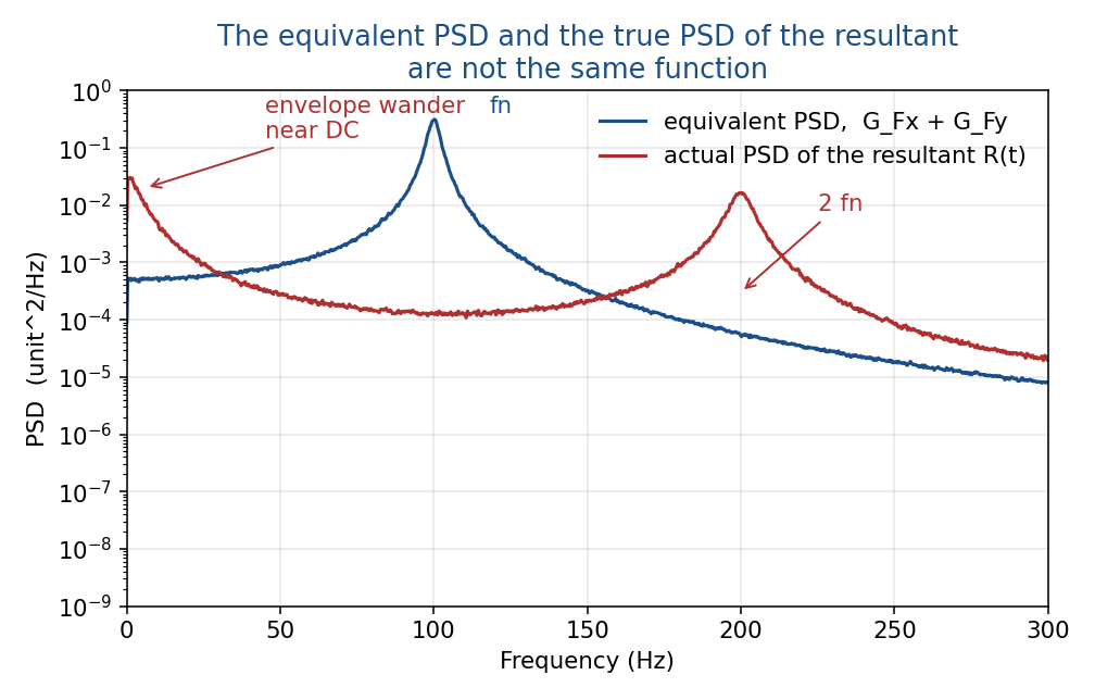
Figure 2. The equivalent PSD and the true spectral density of the resultant occupy different frequency ranges. Neither curve is wrong. They answer different questions.

Both objects have their place. The equivalent PSD is the one that plugs into existing spectral fatigue machinery. The Isserlis result is the one that actually describes the second order behavior of the metric. Difficulty arises only when the first is interpreted as though it were the second.

The Rate of Maxima

A fatigue calculation needs a cycle count, and the cycle count follows from the rate of maxima of the metric, not from the rate of maxima of its components. The squaring operation rectifies the process, so the resultant of two narrowband components centered on the same mode oscillates at approximately twice the natural frequency. In the simulation behind Figure 2, the component $F_X$ produced 108 maxima per second and the resultant produced 203.

This is worth stating plainly because the resultant is often described loosely as an envelope, and a true envelope varies slowly. Figure 3 separates the two. The dashed curve is the genuine analytic envelope of the component, obtained from the Hilbert transform, and it does wander slowly. The resultant is a different object. It rides between zero and that envelope at twice the component frequency.

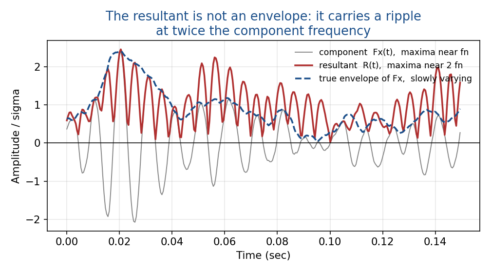
Figure 3. The resultant carries a ripple at twice the component frequency. It is not the slowly varying envelope that the name suggests.

Taking the cycle rate from the equivalent PSD, which peaks at the component natural frequency, therefore under counts cycles for this configuration by roughly a factor of two. When the two directions are dominated by different modes the picture changes again, since beating appears and both sum and difference frequencies enter. There is no single safe rule of thumb here, which is the argument for checking against a synthesized time history.

The Sign Problem

Von Mises stress and resultant shear are nonnegative by construction. Rainflow counting either one directly is meaningless, because every excursion away from zero registers as a range rather than as a reversal, and the alternating and mean components of the resulting cycles have no physical interpretation. The standard remedies are the signed von Mises stress, which attaches the sign of the hydrostatic stress or of the dominant principal stress to the magnitude, and the critical plane methods, which sidestep the issue altogether by projecting the stress tensor onto a candidate plane and retaining a signed scalar. Whichever is chosen, the choice should be stated in the analysis report, because the resulting damage numbers are not interchangeable.

A Recommended Workflow

For a quadratic metric in a random vibration analysis, the following sequence keeps the assumptions visible.

1. Extract the cross spectral density matrix for the response components at the location of interest, not just the individual autospectra. The correlation between components is the quantity that controls everything downstream.

2. Compute the mean square from the trace expression. This step is exact and requires no assumption.

3. Obtain the peak estimate from the generalized chi square distribution rather than from a three sigma rule or from a Rayleigh assumption. Check where the correlation places the case relative to the two limits.

4. If a fatigue number is required, synthesize correlated time histories by Cholesky factoring the cross spectral density matrix at each frequency, evaluate the metric point by point, apply a sign convention, and rainflow the result. This gives the density, the peak distribution, the cycle rate and the damage in a single pass with no distributional assumption.

5. Use the equivalent PSD route for screening and for comparison against legacy results, and treat the synthesized time history as the reference when the two disagree.

References

1. D. Segalman, C. Fulcher, G. Reese, R. Field, An Efficient Method for Calculating RMS von Mises Stress in a Random Vibration Environment, Sandia National Laboratories, SAND98-0260, 1998. Also Journal of Sound and Vibration, 230(2), 2000.

2. A. Preumont, V. Piefort, Predicting Random High Cycle Fatigue Life with Finite Elements, ASME Journal of Vibration and Acoustics, Vol. 116, 1994.

3. X. Pitoiset, A. Preumont, Spectral Methods for Multiaxial Random Fatigue Analysis of Metallic Structures, International Journal of Fatigue, Vol. 22, 2000.

4. J. S. Bendat, A. G. Piersol, Random Data, Analysis and Measurement Procedures, Wiley, New York.

5. J. P. Imhof, Computing the Distribution of Quadratic Forms in Normal Variables, Biometrika, Vol. 48, 1961.

6. R. B. Davies, Algorithm AS 155, The Distribution of a Linear Combination of Chi Squared Random Variables, Applied Statistics, Vol. 29, 1980.

7. R. S. Hoyt, Probability Functions for the Modulus and Angle of the Normal Complex Variate, Bell System Technical Journal, Vol. 26, 1947.

8. L. Isserlis, On a Formula for the Product Moment Coefficient of Any Order of a Normal Frequency Distribution in Any Number of Variables, Biometrika, Vol. 12, 1918.

9. T. Dirlik, Application of Computers in Fatigue Analysis, University of Warwick Thesis, 1985.

Related free ebooks are available at Tom’s Ebooks.