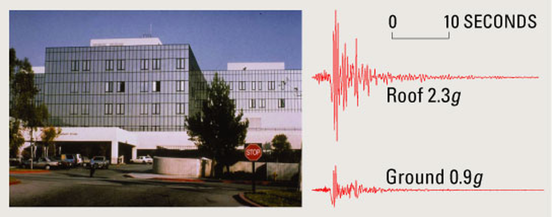
Figure 1. Olive View Hospital, 1994 Northridge earthquake: 0.9 g on the ground, 2.3 g on the roof. Source: USGS Fact Sheet 068-03.
A component bolted to a roof or an upper floor does not feel the earthquake. It feels the floor. The building filters broadband ground shaking into narrowband, nearly harmonic motion at its own natural frequencies, and any equipment tuned near one of those frequencies is driven much as it would be by a sine dwell. The floor response spectrum (FRS), also called the in-structure response spectrum, is the tool that captures this. It is the handoff document between the structural analyst and the equipment qualifier.
I recently posted a revised slide deck on the subject, and a reader wrote with two good follow-up questions: one on the mechanics of generating an FRS from a time-history analysis, and one on which damping ratio to use when scaling ground motion records. This post gives an overview of the slides and then answers both questions.
Download the slides: Earthquake Floor Response Spectra, Revision B (PowerPoint, 41 slides, with speaker notes)
Two Filters in Series
The central idea of the deck is that the building and the equipment are two filters in series. The building is filter number one. It takes broadband ground motion and passes mainly the energy near its own modes. The equipment, modeled as a single-degree-of-freedom oscillator with natural frequency $f_e$ and damping $\zeta_e$, is filter number two.
The absolute acceleration at floor level $k$ is a sum of modal absolute accelerations, weighted by mode shape times participation factor:
$$\ddot{u}_k(t) = \sum_j \phi_{kj}\,\Gamma_j\,\ddot{y}_j(t), \qquad \sum_j \phi_{kj}\,\Gamma_j = 1$$
The floor response spectrum is then simply the shock response spectrum of that floor record:
$$\mathrm{FRS}_k(f_e, \zeta_e) = \max \left| \text{response of an } (f_e, \zeta_e) \text{ SDOF to } \ddot{u}_k(t) \right|$$
Why are tuned floor peaks so large? Ground motion is broadband, so a 5 percent damped oscillator amplifies it only about 2 to 2.5 times. Floor motion near the building fundamental is almost a sinusoid, so a tuned oscillator builds up toward its full amplification factor $Q = 1/(2\zeta)$, which is 10 at 5 percent damping and 25 at 2 percent. The strong-motion duration and the floor’s own bandwidth keep it from reaching the full value, but it gets much closer than it does on the ground.
The Worked Example
Every number in the deck comes from one generic five-story shear building. It is a teaching model, not a real building.
| Property | Value |
|---|---|
| Stories | 5 at 3.6 m, total height 18 m |
| Floor mass | 400 t each, 2,000 t total |
| Story stiffness | 780 MN/m, uniform |
| Building damping | 5 percent modal, linear elastic, fixed base |
| Natural frequencies | 2.00, 5.84, 9.20, 11.82, 13.48 Hz |
| Effective modal mass | 88.0, 8.7, 2.4, 0.8, 0.2 percent |
Two inputs are used. The first is a synthesized record matched to an ASCE 7 style design spectrum ($S_{DS}$ = 1.0 g, $S_{D1}$ = 0.6 g), with a PGA of 0.41 g and its 5 percent spectrum within 0.88 to 1.12 of the target from 0.25 to 50 Hz. The second is the 1940 El Centro north-south record, used unscaled, with a PGA of 0.35 g.
Figure 2 shows what the building does to the synthesized input. The roof record is dominated by a regular half-second cycle, the first mode, and its peak is 1.39 g, 3.4 times the PGA.
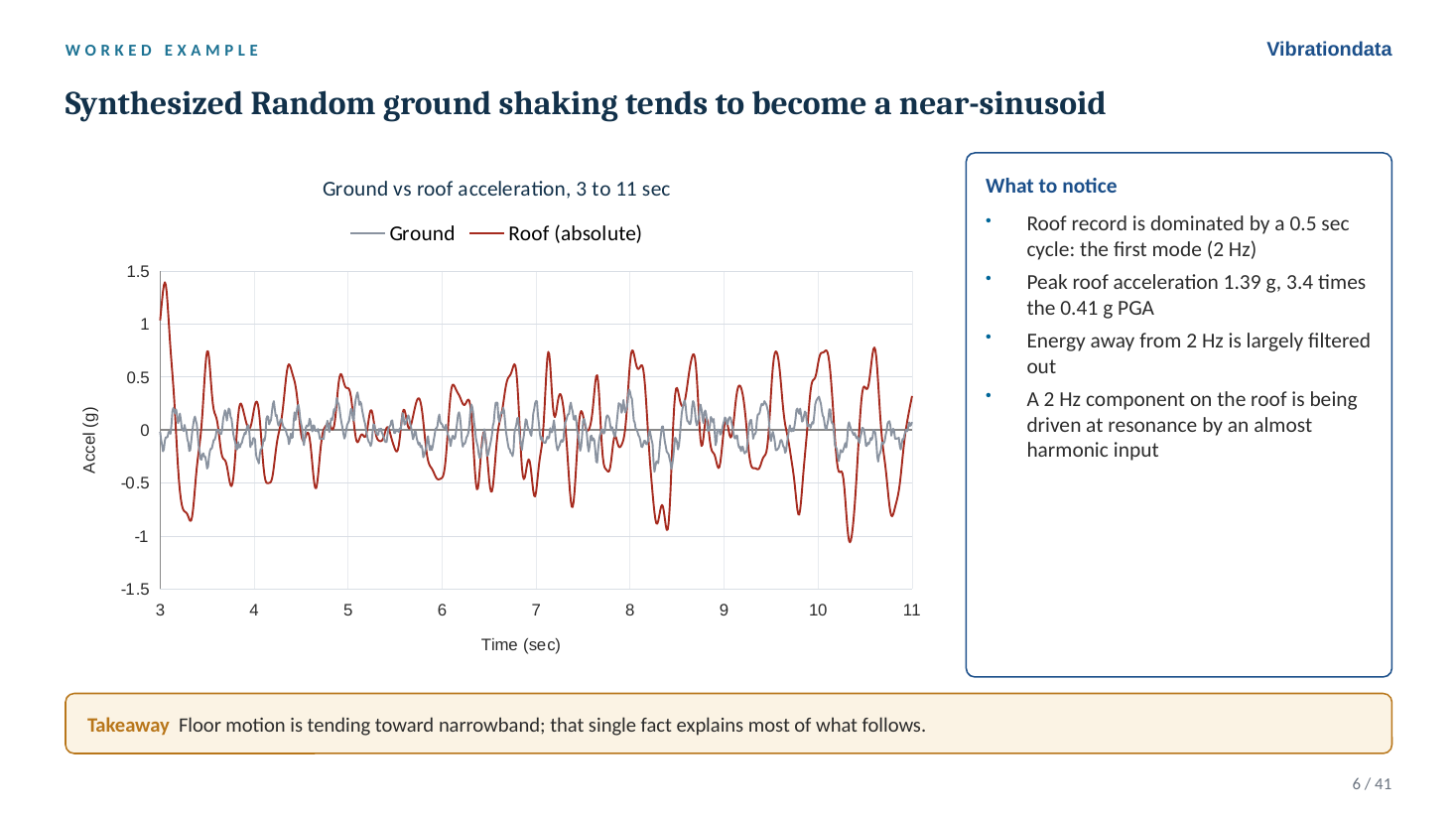
Figure 2. Broadband ground shaking becomes a near-sinusoid at the roof.
Anatomy of a Floor Spectrum
Figure 3 shows the 5 percent floor spectra at every level. Four features are worth reading on any floor spectrum:
- The tuned peak at the fundamental. At the roof it is 5.9 g, against 1.0 g on the ground spectrum at 2 Hz.
- The second-mode peak near 5.7 Hz. At Level 1 this is the largest ordinate on the curve, which is why truncating to one mode is unconservative for low-level equipment.
- Little amplification below the fundamental. At 1 Hz the roof is 1.06 g against 0.62 g on the ground.
- The rigid range. Above the highest building mode the spectrum settles to the peak floor acceleration (the zero period acceleration, ZPA), 1.40 g at the roof. A rigid component simply rides the floor.
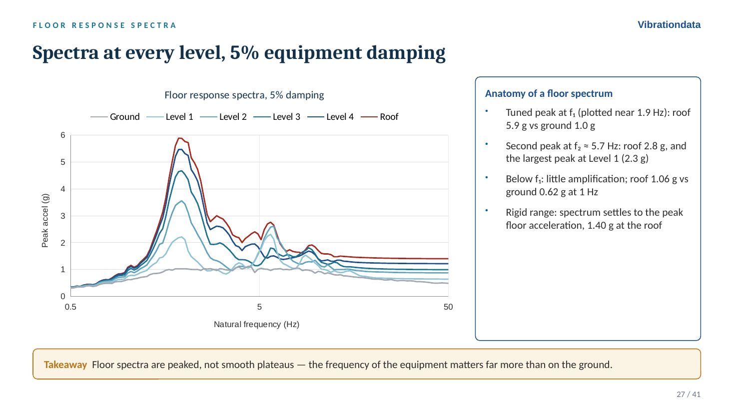
Figure 3. Floor spectra are peaked, not smooth plateaus.
Equipment Damping Matters More on a Floor
Dropping the equipment damping from 5 to 2 percent raises the roof peak from 5.9 g to 9.9 g, a factor of 1.67. The same change on the ground spectrum at 2 Hz is only 1.23. For a pure harmonic input the ratio would be the ratio of the Q values, 25/10 = 2.5. For a long broadband input it would be roughly $\sqrt{2.5} \approx 1.6$. The floor result sits closer to the harmonic case because the floor input is narrowband. An error in equipment damping therefore costs much more on a floor than it does on the ground.
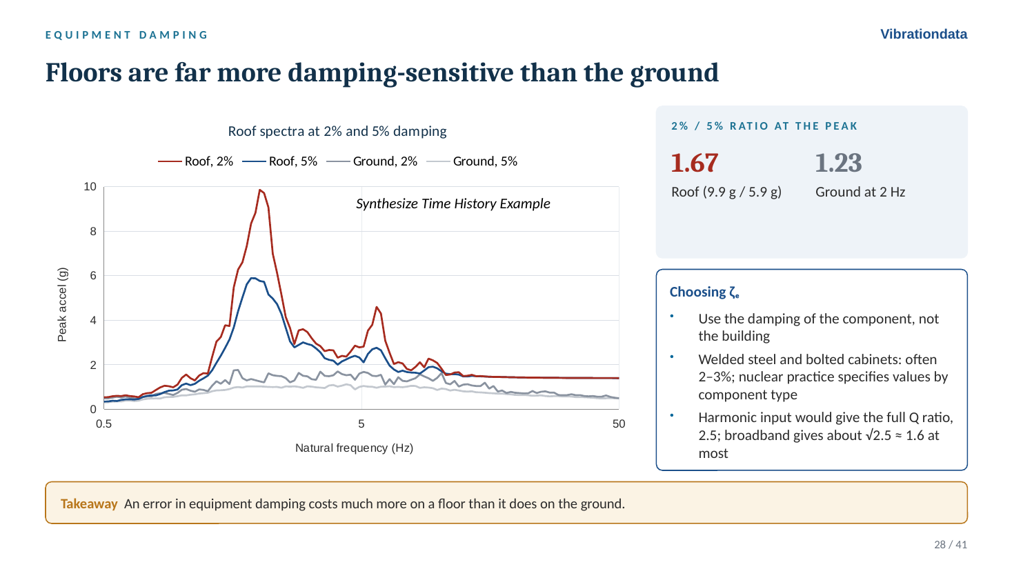
Figure 4. The 2 to 5 percent ratio is 1.67 on the roof versus 1.23 on the ground.
Peak Broadening
A computed floor spectrum has sharp peaks at frequencies set by the building model, and those frequencies are uncertain: concrete cracking, mass and stiffness estimates, soil-structure interaction, nonstructural stiffness, and amplitude-dependent stiffness in strong shaking all move them. ASCE 4-16 broadens each peak by ±15 percent in frequency. USNRC Regulatory Guide 1.122 calls for a minimum of ±10 percent, more if the computed variation warrants. In the example, broadening turns the sharp 9.9 g spike into a 9.9 g plateau from 1.7 to 2.35 Hz. Any equipment in that band must take the peak.
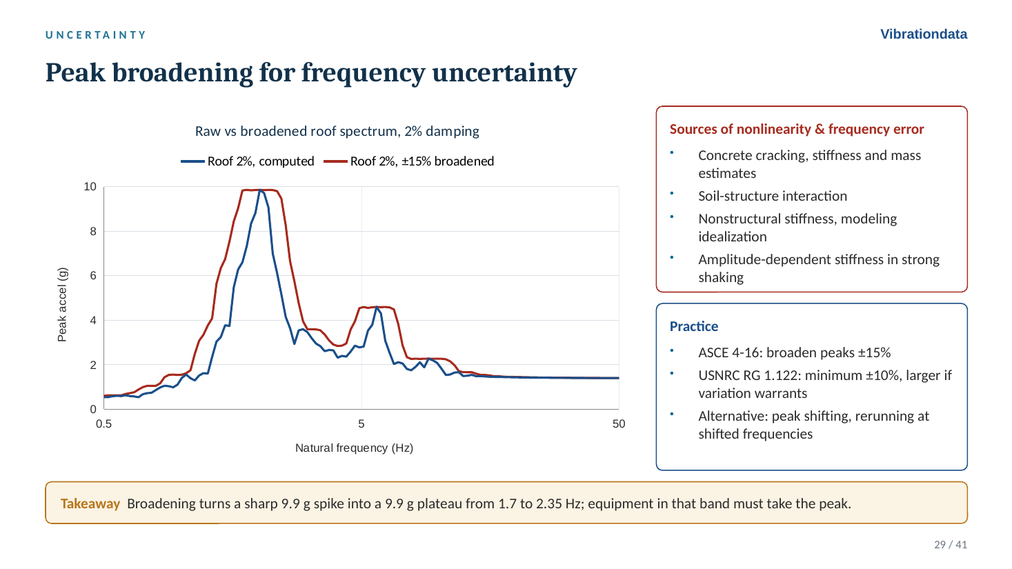
Figure 5. Raw and ±15 percent broadened roof spectra at 2 percent damping.
Doing It in the Vibrationdata App
Slides 7 through 21 walk through the whole calculation in the Vibrationdata Matlab GUI package with the El Centro record. The steps are: import the record from the seismic library, open the shear building tool under Structural Dynamics, enter the floor masses, stiffnesses and heights, check the modal results, set the building damping, apply the record as an arbitrary base input, review the peak floor accelerations, relative displacements, drift ratios and base shear, export the floor acceleration histories, and finally run the SRS tool on the fifth-floor record. That last step is where the equipment damping enters. At Q = 10 the roof spectrum peaks at 4.9 G at 2 Hz. At Q = 25 it peaks at 6.69 G.
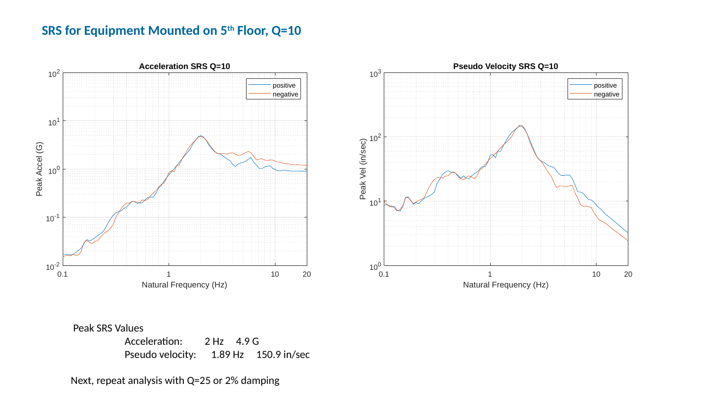
Figure 6. Acceleration and pseudo velocity SRS of the fifth-floor response to El Centro, Q = 10.
Note the pseudo velocity spectrum alongside the acceleration spectrum: 150.9 in/sec at Q = 10 and 223.5 in/sec at Q = 25. Acceleration spectra dominate seismic practice, but pseudo velocity is the better indicator of damage potential, since stress in a structure or component is proportional to velocity through $\sigma = \rho c V$. Plotting both often changes the impression of which input or which floor is the more severe. My free ebooks develop the stress-velocity relationship in detail.
Same Building, Two Inputs
Running El Centro through the same building separates what the building controls from what the record controls.
| Quantity | Synthesized | El Centro NS |
|---|---|---|
| PGA | 0.41 g | 0.35 g |
| Ground 5% SA at f1 | 1.0 g | 0.84 g |
| Roof PFA / PGA | 3.39 | 3.33 |
| Roof 5% peak | 5.9 g | 4.9 g |
| Roof 5% peak / ground SA at f1 | 5.9 | 5.8 |
| Roof 2% peak | 9.9 g | 6.9 g |
| Roof 2% / 5% ratio | 1.67 | 1.41 |
| Level 1 governing peak | mode 2, 2.3 g | mode 1, 1.6 g |
| Roof displacement | 80 mm | 65 mm |
The shaded ratios are set by the building and carry over almost exactly between the two records. The others move with the record. The damping ratio and which mode governs a low floor both changed. That is the practical argument for using several records and averaging or enveloping them, rather than trusting one.
Roof Equipment: Mount It Stiff
Figure 7 overlays the roof spectra from both inputs at 2 and 5 percent damping and shades the frequency bands that matter for design. Above about 20 Hz, beyond the highest building mode, a rigid item rides the floor at 1.2 to 1.4 g. Near the building fundamental, 1.5 to 2.5 Hz after broadening, a lightly damped item sees 7 to 10 g. The second mode adds a smaller peak of 2.3 to 4.5 g between 5 and 7 Hz.
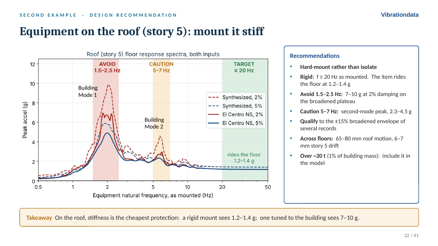
Figure 7. On the roof, stiffness is the cheapest protection.
Rooftop units on spring isolators are the classic trap. Isolators commonly sit at 2 to 5 Hz, which can land the equipment right on the building fundamental or second mode. They need seismic restraints and snubbers. Piping and conduit that cross floors must also accommodate the relative motion, 65 to 80 mm at the roof in this example.
Code Practice and Measured Buildings
ASCE 7-22 Section 13.3.1.1 introduced a height amplification factor that replaced the old linear $1 + 2z/h$:
$$H_f = 1 + a_1\left(\frac{z}{h}\right) + a_2\left(\frac{z}{h}\right)^{10}, \qquad a_1 = \frac{1}{T_a} \le 2.5, \qquad a_2 = 1-\left(\frac{0.4}{T_a}\right)^2 \ge 0$$
With $T_a$ = 0.5 sec, $H_f$ at the roof is 3.36, against 3.39 computed for the elastic building. The old linear form gives 3.0. The component force equation then reads naturally as a simplified floor spectrum, PGA times height amplification times resonance amplification:
$$F_p = 0.4\,S_{DS}\,I_p\,W_p\left(\frac{H_f}{R_\mu}\right)\left(\frac{C_{AR}}{R_{po}}\right)$$
In the elastic example the ratio of floor spectrum peak to peak floor acceleration is 4.2 at 5 percent damping and 7.1 at 2 percent, well above the tabulated $C_{AR}$ values. That is not a code error. The table carries ductility and statistical assumptions. But it marks where the simplified method is least appropriate: rigid or brittle anchorage, or functionally critical equipment tuned to a building mode. For those, Chapter 13 permits floor spectra from building analysis.
The deck also tabulates measured roof-to-ground ratios from 18 instrumented buildings, from a 3-story store to the Transamerica Pyramid. The median is 1.9, the range 0.75 to 3.1, with no trend in story count. The four structurally damaged buildings all fall between 0.75 and 1.7, which is the effect $R_\mu$ represents. The 1994 Northridge record at Olive View Hospital in Figure 1, 0.91 g free field and 2.31 g at the roof, is a vivid example of site frequency and building frequency nearly coinciding: the building fundamental was estimated at 2.5 Hz, and the soil-driven foundation motion was concentrated in the 2 to 3 Hz range.
Heavy Equipment Talks Back
The floor spectrum assumes the equipment does not affect the floor. Attaching a 2 percent damped oscillator tuned to the 2 Hz roof mode shows how quickly that assumption fails. The decoupled FRS gives 10.4 g. At a mass ratio of 0.1 percent, the coupled peak is 12 percent lower. At 1 percent it is 38 percent lower, and the tuned pair splits into modes at 1.87 and 2.14 Hz, the tuned mass damper effect. At 10 percent it is 70 percent lower.
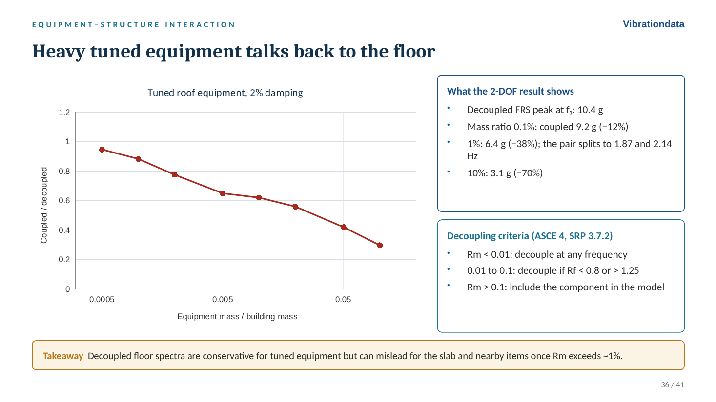
Figure 8. Coupled versus decoupled response for tuned roof equipment.
The ASCE 4 and SRP 3.7.2 criteria use the mass ratio $R_m$ and frequency ratio $R_f$: decouple at any frequency for $R_m$ below 0.01; decouple for $R_m$ from 0.01 to 0.1 only if $R_f$ is below 0.8 or above 1.25; include the component in the model above 0.1. Decoupling is conservative for the tuned item itself, but the split modes shift the floor spectrum for other items on the same floor.
The remaining slides cover three-direction demands and slab vertical modes, seismic anchor motion as a separate load case, the 100-40-40 combination rule with a worked anchor-bolt example, qualification by analysis and by shake-table test (IEEE 344 and ICC-ES AC156), and a checklist of common mistakes.
Reader Question 1: Generating the FRS from Time-History Analysis
When developing an FRS from a time-history analysis, you would first run the THA on your building model, record the absolute acceleration response history at a floor node, and then use the expected damping ratio of the equipment to generate the FRS. For equipment with 2 percent damping, you would use 2 percent when converting the floor acceleration time history into a response spectrum. The building’s damping is already accounted for in the floor nodal acceleration history. Is that correct?
Yes, that is correct.
- Run the time-history analysis (THA) on the building model, with the building’s own damping.
- Record the absolute acceleration history at the floor node, not the acceleration relative to the base. An oscillator mounted on the floor responds to the floor’s total motion.
- Compute the SRS of that history using the equipment damping, 2 percent in this example.
The building damping is already embedded in the floor response, so it is not applied a second time. It is common to generate the FRS at several damping values, say 2, 3 and 5 percent, so the equipment analyst can pick the appropriate curve. Figure 4 shows why the choice deserves care. A few practical points go with the procedure:
- Broaden the peaks. Broaden by ±15 percent per ASCE 4-16, or at least ±10 percent per RG 1.122. A sharp unbroadened peak is unconservative if the real building frequency shifts slightly.
- Use multiple records and all three directions. Average or envelope per the governing standard. The two-input comparison above shows how much a single record can mislead.
- Watch Rayleigh damping. If the building model uses Rayleigh damping, the stiffness-proportional term can heavily overdamp the higher modes. That suppresses high-frequency floor content and can make the FRS unconservative in the range where much equipment lives. Check the effective damping at those frequencies.
- Check the decoupling assumption. If the equipment mass is significant and its frequency is near a building mode, couple it into the building model, per the $R_m$ and $R_f$ criteria above.
- Resolve the frequencies. The THA time step, output rate and SRS calculation all need to resolve the highest frequency of interest, at least 10 samples per cycle, or a ramp-invariant SRS filter. In the deck, El Centro’s 100 samples/sec was upsampled to 1000 samples/sec before running the building and spectra.
Reader Question 2: Which Damping for Scaling Ground Motions?
Some argue that records should always be scaled to a 5 percent damped target spectrum, regardless of the building’s expected damping. Others believe the target should use the expected damping ratio of the building. I tend to side with the former, because the purpose is to select and scale records, not to use the resulting spectrum for design. The building’s damping will already be accounted for in the subsequent time-history analysis, and a 5 percent target avoids the uncertainty of damping modification factors. Do you have a preference?
I agree: scale to the 5 percent damped target. Three reasons:
- The hazard is defined at 5 percent. Ground motion models, and the design spectra built from them such as the ASCE 7 MCER spectrum, are 5 percent damped. The 5 percent spectrum is the intensity measure the hazard actually describes. Selection and scaling are about matching that hazard, not about designing the building.
- Damping modification factors add uncertainty. The ratio between a 2 percent and a 5 percent spectrum is not a universal constant. It depends on period and on duration, or number of cycles, with long-duration records showing a larger ratio. The deck shows a version of this directly: the 2/5 percent ratio was 1.23 on the ground but 1.67 on the roof, and 1.67 versus 1.41 between two records at the same roof. Converting the target to 2 percent with a generic factor introduces a bias that has nothing to do with the hazard.
- Building damping belongs in the structural model. It is captured where it physically acts, in the THA. Putting it into the target spectrum as well mixes two separate things.
One caveat. If you use spectral matching, such as wavelet adjustment, rather than amplitude scaling, a good match at 5 percent does not guarantee the same quality of match at other damping values. It is worth plotting the matched records at 2 percent to make sure nothing unusual happens, particularly if floor spectrum or equipment work will follow.
Summary
- The building is the first filter. Floor motion is narrowband, peaked and damping-sensitive, so treat it as such rather than as ground motion.
- In the example, roof PFA was 3.4 times PGA, and the ASCE 7-22 $H_f$ matched it at the roof (3.36 versus 3.39).
- A tuned roof component saw 5.9 g at 5 percent damping and 9.9 g at 2 percent, against 1.0 g on the ground spectrum.
- Broaden the peaks, use several records, keep enough modes to reach the rigid range, and include heavy equipment in the model.
- Generate the FRS from the absolute floor acceleration at the equipment damping. Scale the ground motions to the 5 percent hazard spectrum.
The full deck, with speaker notes on every slide, is here: Earthquake_Floor_Response_Spectra_revB.pptx.
References
- ASCE/SEI 7-22, Chapter 13: Seismic Design Requirements for Nonstructural Components
- ASCE/SEI 4-16, Seismic Analysis of Safety-Related Nuclear Structures
- USNRC Regulatory Guide 1.122, Development of Floor Design Response Spectra
- USNRC SRP 3.7.2, Seismic System Analysis
- IEEE 344, Seismic Qualification of Equipment for Nuclear Power Generating Stations
- ICC-ES AC156, Seismic Certification by Shake-Table Testing of Nonstructural Components
- Smallwood, D.O., An Improved Recursive Formula for Calculating Shock Response Spectra, 1981
- Singh, M.P., Generation of Seismic Floor Spectra, J. Eng. Mech. Div., ASCE, 1975
- USGS Fact Sheet 068-03 (Olive View Hospital, 1994 Northridge)
See also my free ebooks on shock and vibration response spectra and the stress-velocity relationship.