A reader has a measured time history, he wants a low-frequency sine test level from it, and the FFT does not seem to give him the real amplitude at each frequency. His governing handbook sends him to something called ESI, which produces a swept sine test that he suspects is too severe at the natural frequencies of his structure. Is there a better way to get the right amplitude at the right frequency?
ESI stands for Equivalent Sine Input. The term is standard in ECSS documents and in the Ariane and Vega user community. It is much less common in the United States, even though American programs do essentially the same thing under other names. This post explains what ESI is, shows that it is exact in the one sense it claims to be, and then locates where the overtest really comes from. The answer is not where most people look first.
Spacecraft see low-frequency transients during launch: liftoff, engine ignition and cutoff, stage separation, gusts. These are predicted by a coupled loads analysis (CLA) of the launcher and spacecraft together, or measured in flight. Spacecraft are qualified on a shaker with a swept sine, typically 5 to 100 Hz. ESI is the bridge between the two.
What ESI Is
The recipe has three steps. Take the acceleration time history at the launcher-to-spacecraft interface. Compute its shock response spectrum at a chosen amplification factor Q. Divide by Q.
$$\mathrm{ESI}(f_n)=\frac{\mathrm{SRS}(f_n,Q)}{Q}$$
The logic is simple. A single-degree-of-freedom (SDOF) system driven at its natural frequency by a steady sine of amplitude $A$ responds with amplitude $A\sqrt{Q^2+1}$, which is $QA$ for any practical Q. So a sine of amplitude SRS/Q produces the same peak response that the transient produced, in an oscillator of that frequency and that Q. Repeat at every natural frequency and the result is a sine amplitude spectrum.
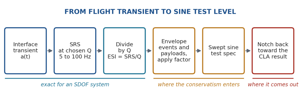
Figure 1. The ESI process. The first three steps are an exact equivalence for an SDOF system. The conservatism enters when the curves are enveloped and squared off into a test specification, and it is removed again by notching.
ECSS-E-HB-32-26A, the Spacecraft Mechanical Loads Analysis Handbook, is the reference. Calvi’s overview paper notes that the ESI is usually computed from the CLA time histories at two damping values, Q of 20 and Q of 50, because the damping of the test article is not known in advance. The reason two values are needed will become clear below.
A Worked Example
The example is a generic two-mass model. It is an illustration and does not represent any launcher or spacecraft. One mass on a grounded spring stands for a launcher mode. A second mass on top stands for the spacecraft and its fundamental axial mode. A thrust transient is applied to the lower mass, and the acceleration of the lower mass is the interface acceleration.
Table 1. Coupled Model
| Parameter | Value |
|---|---|
| Launcher modal mass and uncoupled frequency | 20,000 kg, 18 Hz, Q = 15 |
| Spacecraft mass and fixed-base frequency | 2,000 kg, 35 Hz, Q = 25 |
| Coupled natural frequencies | 16.9 Hz and 37.2 Hz |
| Forcing | 400 kN thrust change over 15 msec, versed sine ramp |
| Sample rate, record length | 4000 samples/sec, 3 sec |
| Peak interface acceleration | 1.45 G |
| Peak spacecraft response | 3.36 G |
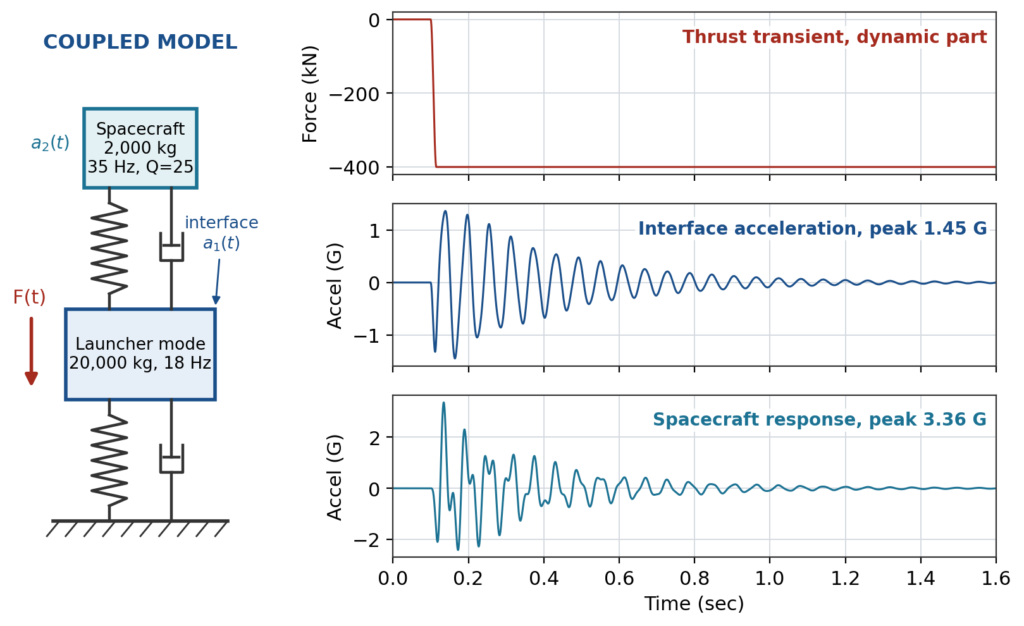
Figure 2. The coupled model and its response to the thrust transient. The interface acceleration is dominated by the 16.9 Hz coupled mode. The spacecraft response carries both coupled modes.
Note that the two coupled frequencies are 16.9 and 37.2 Hz. Neither one is the spacecraft fixed-base frequency of 35 Hz. That detail matters later.
SRS and ESI at Four Values of Q
The SRS of the interface acceleration was computed with the Smallwood ramp invariant digital recursive filtering relationship at 1/24 octave spacing from 5 to 100 Hz.
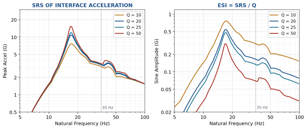
Figure 3. Left: SRS of the interface acceleration. Right: the same curves divided by Q. The SRS grows with Q, but much more slowly than Q itself, so the ESI falls as Q rises.
Table 2. SRS and ESI at Two Frequencies
| Q | SRS at 16.9 Hz (G) | ESI at 16.9 Hz (G) | SRS at 35 Hz (G) | ESI at 35 Hz (G) |
|---|---|---|---|---|
| 10 | 7.59 | 0.759 | 3.08 | 0.308 |
| 20 | 10.87 | 0.544 | 3.31 | 0.165 |
| 25 | 12.01 | 0.481 | 3.36 | 0.134 |
| 50 | 15.57 | 0.311 | 3.47 | 0.069 |
At 16.9 Hz the oscillator is tuned to the dominant frequency in the input, and a fivefold increase in Q raises the SRS by a factor of 2.05. At 35 Hz the oscillator is not tuned to anything in the input, and the same fivefold increase in Q raises the SRS by only 13 percent. In both cases the SRS is far from proportional to Q. A few cycles of a decaying transient cannot pump a lightly damped oscillator up to its steady-state amplification.
The Equivalence Is Exact for an SDOF System
Look at the Q = 25 row of Table 2. The SRS at 35 Hz is 3.36 G. That is the peak spacecraft response from Table 1, to three figures. This is no coincidence. The spacecraft in this model is an SDOF system at 35 Hz with Q = 25 sitting on the interface, so its response to the interface motion is exactly what the SRS calculates. The ESI at 35 Hz and Q = 25 is 0.134 G, and 0.134 G times 25 is the flight response.
As a further check, a swept sine with its amplitude following the Q = 25 ESI curve was applied to a 35 Hz, Q = 25 oscillator at 2 octaves/minute. The peak response was 3.28 G, or 98 percent of the 3.36 G flight value. The missing 2 percent is the sweep rate effect discussed below.
The raw ESI is not conservative. For an SDOF system with the assumed Q, a sine at the ESI level reproduces the flight peak response, no more and no less. It also accounts for the whole input. The SRS at 35 Hz is 3.36 G even though the interface acceleration has almost no Fourier content at 35 Hz, because the oscillator responds to the 16.9 and 37.2 Hz content too.
Why Not Read the Amplitude off the FFT?
The FFT does not lose the amplitude. It is a matter of scaling, and the convention varies from one software package to the next. For N points, the one-sided peak amplitude at spectral line k is
$$A_k=\frac{2}{N}\left|X_k\right|$$
with the factor of 2 omitted at zero frequency. A 1 G sine at 20 Hz then reads 1 G at 20 Hz, provided 20 Hz falls on a spectral line. Between lines the reading is low by up to 36 percent with a rectangular window and 15 percent with a Hanning window after its amplitude correction. A flat top window holds the error to a fraction of a percent.
But that scaling is meaningful only for a sine that persists over the entire record. For a transient it is not. Table 3 shows the interface acceleration from the example, analyzed as recorded and again with zeros appended to double and quadruple the record length. The event has not changed.
Table 3. Effect of Record Length on the 16.9 Hz Peak
| Record length | FFT x 2/N (G peak) | Fourier transform (G-sec) | SRS, Q = 20 (G) |
|---|---|---|---|
| 3 sec | 0.166 | 0.249 | 10.87 |
| 6 sec | 0.083 | 0.249 | 10.87 |
| 12 sec | 0.042 | 0.252 | 10.87 |
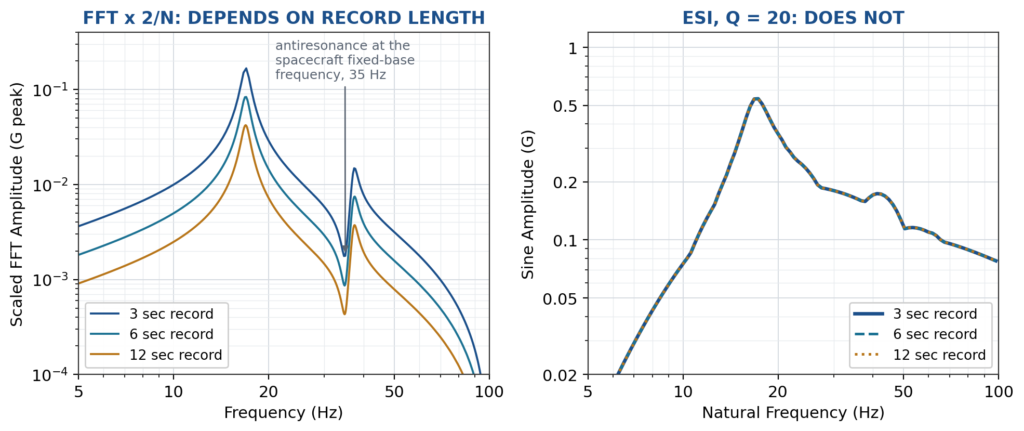
Figure 4. The scaled FFT of a transient falls in proportion to the record length. The ESI is unchanged. Note the antiresonance in the interface acceleration at 35 Hz, the spacecraft fixed-base frequency.
The amplitude-scaled FFT halves every time the record doubles. There is no “real amplitude at each frequency” for a transient. The proper Fourier quantity is the transform scaled by the time step, with units of G-sec, which is a density and is independent of record length. It is a legitimate descriptor, and it has a classical connection to the SRS: for an undamped oscillator, the residual response after the input has ended is $2\pi f_n$ times the Fourier transform magnitude at $f_n$. But it says nothing about damping or about the peak reached while the input is still acting. The SRS answers the question the test engineer is really asking, which is what the input does to a resonant system.
Where the Conservatism Comes From
1. Q Mismatch
Steady-state sine response is proportional to Q. Transient response is not. So if the ESI is computed at an assumed value $Q_a$ and the test article has a true value $Q_t$, the ratio of sine test response to flight response is
$$\frac{\text{sine response}}{\text{flight response}}=\frac{Q_t}{Q_a}\,\frac{\mathrm{SRS}(f_n,Q_a)}{\mathrm{SRS}(f_n,Q_t)}$$
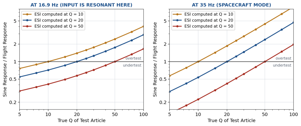
Figure 5. Ratio of sine test response to flight response when the ESI is computed at one Q and the test article has another. Left: at the dominant input frequency. Right: at the spacecraft mode, where the SRS barely depends on Q and the error is nearly proportional to the Q ratio.
Computing the ESI at Q = 10 for an article that really has Q = 30 gives an overtest of 1.8 at 16.9 Hz and 2.7 at 35 Hz. The error runs both ways. Computing at Q = 50 for an article with Q = 20 is an undertest by a factor of 0.57 and 0.42 respectively. This is why the European practice carries two curves, Q = 20 and Q = 50. The low-Q curve is the conservative one for setting a test level. The curve nearest the measured damping is the right one for justifying a notch. The damping is measured in the low-level sine run that precedes the full-level run, so the choice can be checked before it matters.
2. Enveloping, and the Peak That the Payload Never Sees
A launcher user manual does not give one ESI curve. It gives a simple specification meant to cover many events and many payloads. To imitate that, the coupled model was run 54 times: spacecraft frequencies of 25, 30, 35, 40, 45 and 50 Hz, spacecraft masses of 1000, 2000 and 4000 kg, and thrust ramp times of 10, 15 and 25 msec.
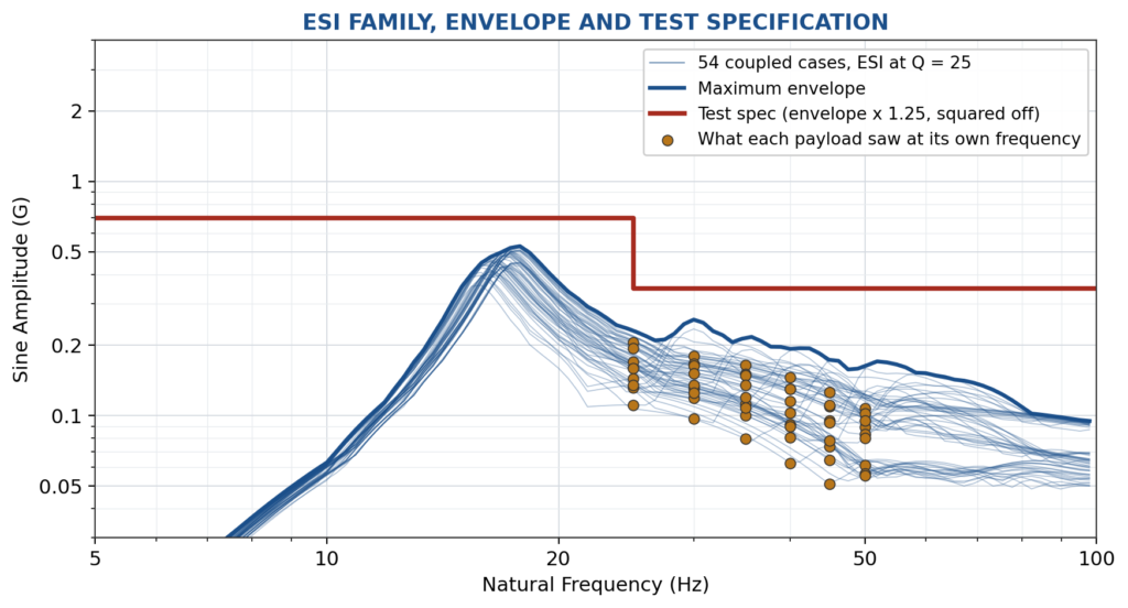
Figure 6. ESI curves at Q = 25 for 54 coupled cases, their maximum envelope, and a two-level test specification set at 1.25 times the envelope and squared off. The markers show the ESI that each payload experienced at its own fixed-base frequency.
Every marker in Figure 6 lies below the maximum envelope, and far below the specification. This is the vibration absorber effect. At its own fixed-base frequency a spacecraft pushes back on the launcher and creates an antiresonance in the interface motion, as Figure 4 showed at 35 Hz. The coupled system peaks occur at frequencies shifted away from the fixed-base frequency. Move the spacecraft frequency and the coupled peak moves with it, always staying out of reach. The envelope is built from peaks that belong to other payloads. Then the shaker, which has effectively infinite impedance, enforces that level exactly where the test article is most responsive.
Table 4. How 0.134 G Became 0.35 G at 35 Hz
| Step | Level (G) | Factor |
|---|---|---|
| ESI of this payload’s own coupled analysis, Q = 25 | 0.134 | – |
| Maximum envelope of the 54-case family | 0.213 | 1.59 |
| Qualification factor of 1.25 | 0.266 | 1.25 |
| Squared off to a two-level specification | 0.35 | 1.31 |
| Total | 2.6 |
3. Cycles
The unnotched specification was applied to the 35 Hz, Q = 25 spacecraft mode as a logarithmic sweep from 5 to 100 Hz.
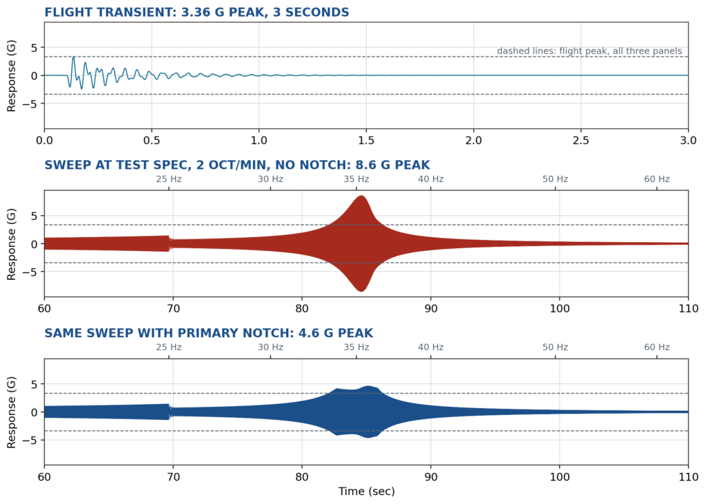
Figure 7. Spacecraft response. Top: the flight transient. Middle: the sweep at the unnotched specification. Bottom: the same sweep with a primary notch. The sweep panels show a 50 second window around resonance. The dashed lines mark the flight peak.
Table 5. Response Peaks, Counting Both Polarities
| Case | Peak (G) | Peaks at or above 50% of flight peak | At or above 90% | Relative damage, b = 6.4 |
|---|---|---|---|---|
| Flight transient | 3.36 | 6 | 1 | 1 |
| Sweep at raw ESI, 2 oct/min | 3.28 | 210 | 59 | 48 |
| Sweep at specification, 2 oct/min | 8.56 | 623 | 329 | 22,000 |
| Sweep at specification, 4 oct/min | 8.29 | 311 | 157 | 10,200 |
| Notched sweep, 2 oct/min | 4.63 | 623 | 329 | 890 |
The relative damage is the sum of the response peaks raised to a fatigue exponent of 6.4, normalized to the flight event. It is a relative index only. The point is the first two rows. Even a sweep at the raw ESI level, which matches the flight peak, delivers 48 times the damage because the transient visits its peak once and the sweep lingers there. In a logarithmic sweep at R octaves/minute the number of cycles spent within the half-power bandwidth is approximately
$$N\approx\frac{60\,f_n}{R\,Q\,\ln 2}$$
which is 61 cycles for 35 Hz, Q = 25 and 2 octaves/minute. ESI is a peak response equivalence. It was never a fatigue equivalence. For most spacecraft primary structure that is acceptable, since the design is governed by strength and stability. For mechanisms, bonded joints and anything with a short fatigue life it deserves a separate look.
4. Sweep Rate
A sweep does not quite reach steady state. Table 6 gives the peak response as a fraction of the steady-state value, from numerical simulation with a constant-amplitude logarithmic sweep.
Table 6. Peak Sweep Response as a Fraction of Steady State
| Natural frequency | Q | 2 oct/min | 4 oct/min |
|---|---|---|---|
| 5.5 Hz | 25 | 0.84 | 0.74 |
| 5.5 Hz | 50 | 0.63 | 0.52 |
| 17 Hz | 25 | 0.95 | 0.89 |
| 17 Hz | 50 | 0.81 | 0.71 |
| 35 Hz | 25 | 0.98 | 0.95 |
| 35 Hz | 50 | 0.89 | 0.81 |
This works against the other three items, and it is significant only for lightly damped modes at the bottom of the band. A faster sweep halves the cycle count and trims the peak slightly. Whether the faster rate is allowed is set by the specification, commonly 2 octaves/minute for qualification and 4 octaves/minute for acceptance.
Notching
The remedy is to reduce the input in a narrow band around the resonance so that the response, or better the interface force and moment, does not exceed what the coupled analysis predicts with margin. This is primary notching. Secondary notching does the same for equipment responses inside the spacecraft. For the example, the input was limited so that the steady-state response stays at or below 1.25 times the flight value:
$$A_{notch}(f)=\min\left[A_{spec}(f),\;\frac{1.25\,a_{flight}}{\left|T(f)\right|}\right]$$
where $T(f)$ is the transmissibility of the 35 Hz mode.
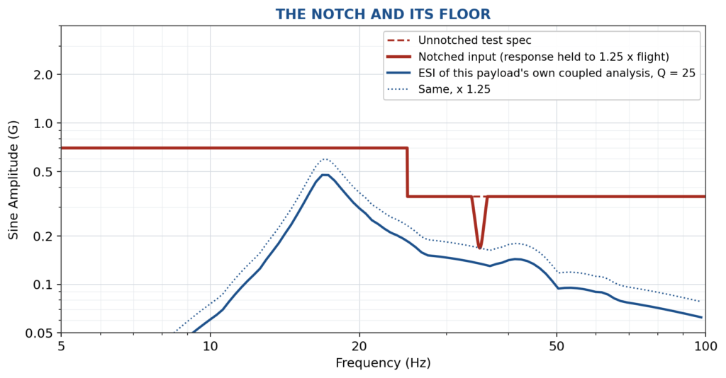
Figure 8. The notched input compared with the ESI of this payload’s own coupled analysis. The bottom of the notch touches 1.25 times the ESI at 35 Hz. That is the floor.
The notch bottoms out at 0.168 G, a reduction of 6.4 dB from the 0.35 G specification. And 0.168 G is exactly 1.25 times the ESI of 0.134 G. This is the second job that ESI does, and arguably the more important one. The launch authority will accept a notch provided the notched input stays above the ESI from the CLA for that spacecraft, with the agreed factor. ESI creates part of the overtest, and ESI is also the yardstick that justifies removing it.
One caution from the simulation. The notch profile was computed from steady-state transmissibility, but the simulated response reached 4.63 G against a 4.20 G target, a 10 percent overshoot on the way out of the notch. The input amplitude changes rapidly across a narrow notch, and the oscillator is still ringing from the higher level it saw a moment before. Real controllers notch in closed loop on response channels and have their own compression-speed lag, so some overshoot should be expected and the limit set accordingly.
Notching limits the peak, not the cycle count. In Table 5 the notched sweep has the same number of peaks above the flight-based thresholds as the unnotched sweep. The damage index drops by a factor of 25 because the peaks are lower, not because there are fewer of them.
The American Equivalents
American practice reaches the same place by other roads. Low-frequency transients are covered by a sine sweep or a sine burst with levels derived from the coupled loads analysis, often through the SRS of the CLA transients in the same way, without the ESI label. The overtest at resonance is handled by response limiting to CLA predictions and by force limiting, where the interface force is measured and capped. Force limiting addresses the impedance mismatch directly, which is the root of item 2 above.
Summary
- ESI = SRS/Q. It is the sine amplitude that gives an SDOF system of that frequency and Q the same peak response as the transient.
- On those terms it is exact. In the example it reproduced the 3.36 G flight response to within the 2 percent sweep-rate effect.
- An amplitude-scaled FFT of a transient depends on the record length and cannot supply a sine test level. The SRS does not have that problem.
- The SRS grows more slowly than Q, so the ESI must be computed at a Q close to that of the test article. A factor of 3 error in Q produced a factor of 1.8 to 2.7 error in response.
- The main overtest comes from enveloping across payloads and then enforcing the envelope on a rigid shaker. A spacecraft suppresses the interface motion at its own fixed-base frequency in flight. In the example this, the qualification factor and the squaring-off added up to 2.6.
- Notch back to the ESI of the spacecraft’s own coupled analysis, times the agreed factor. That is both the remedy and the floor.
- ESI matches peaks, not cycles. A sweep at the raw ESI level delivered 48 times the fatigue damage index of the flight transient.
- If the verification is by analysis and not by test, skip ESI and apply the time history directly in a modal transient solution.
References
- ECSS-E-HB-32-26A, Spacecraft Mechanical Loads Analysis Handbook, European Cooperation for Space Standardization, 19 February 2013.
- A. Calvi, A Handbook for Spacecraft Structural Dynamics and Loads Analysis, Proceedings of ISMA 2012, Leuven.
- ECSS-E-HB-32-25A, Mechanical Shock Design and Verification Handbook, 14 July 2015.
- D. Smallwood, An Improved Recursive Formula for Calculating Shock Response Spectra, Shock and Vibration Bulletin, No. 51, 1981.
- T. Irvine, Shock and Vibration Response Spectra, free ebook: Tom’s Ebooks.
Tom Irvine, Vibrationdata
Explore more in our Spacecraft Dynamics Knowledge Hub:
View All Spacecraft Dynamics Resources →