Image credit: Nikhil Patil
Introduction
Most vibration-induced fatigue problems in aerospace and industrial structures live comfortably in the high cycle fatigue (HCF) regime, where nominal stresses remain below yield and the stress-life (S-N) method with rainflow cycle counting serves well. But some of the most consequential failures occur in the opposite corner of the map: low cycle fatigue (LCF), where local stresses approach or exceed the yield limit and plastic strain governs the damage. Thermal cycling of engine components, seismic loading of piping and equipment, pressure vessel startup-shutdown cycles, launch vehicle transients, and severe notch plasticity all fall in this category.
When plasticity enters the picture, stress ceases to be the honest damage metric. Two load histories can produce the same nominal stress while producing very different plastic strains. The strain-life (ε-N) method, developed in the 1950s and 1960s from the work of Coffin, Manson, Basquin, Morrow, and Neuber, addresses this by making local strain the damage parameter. This post reviews the strain-life framework and then turns to a phenomenon that the basic method does not capture on its own: ratcheting, the cycle-by-cycle accumulation of directional plastic strain.
HCF versus LCF Regimes
| High Cycle Fatigue | Low Cycle Fatigue | |
|---|---|---|
| Typical life | > 104–105 cycles | < 103–104 cycles |
| Dominant strain | Elastic | Plastic |
| Stress level | Below yield (nominally) | At or above yield |
| Damage parameter | Stress amplitude | Strain amplitude |
| Method | S-N (Basquin), Miner’s rule | ε-N (Coffin-Manson-Basquin) |
| Typical drivers | Random vibration, acoustics, rotating machinery | Thermal cycles, seismic, pressure cycles, severe transients |
The boundary is not a hard wall. The strain-life equation spans both regimes in a single expression, which is one of its principal attractions.
Cyclic Stress-Strain Behavior
A metal cycled into the plastic range does not retain its monotonic stress-strain curve. Depending on its initial condition, it cyclically hardens (typically soft, annealed materials) or cyclically softens (typically cold-worked or quenched-and-tempered materials) until it reaches a stabilized hysteresis loop. A useful rule of thumb: materials with an ultimate-to-yield ratio above about 1.4 tend to harden, and those below about 1.2 tend to soften.
The locus of stabilized loop tips is the cyclic stress-strain curve, usually fit with a Ramberg-Osgood form:
\[ \varepsilon_a = \frac{\sigma_a}{E} + \left( \frac{\sigma_a}{K’} \right)^{1/n’} \]where \( K’ \) is the cyclic strength coefficient and \( n’ \) is the cyclic strain hardening exponent. For many metals \( n’ \approx 0.10 \) to \( 0.20 \). Under Massing’s hypothesis, the stabilized hysteresis loop branch is the cyclic curve magnified by a factor of two in both stress and strain:
\[ \Delta\varepsilon = \frac{\Delta\sigma}{E} + 2\left( \frac{\Delta\sigma}{2K’} \right)^{1/n’} \]These relations allow the analyst to trace hysteresis loops through an arbitrary load history, applying the material memory rules that make rainflow cycle counting physically meaningful: rainflow pairs are precisely the closed hysteresis loops.
The Strain-Life Equation
The total strain amplitude is split into elastic and plastic parts, each following a power law in reversals to failure \( 2N_f \). Basquin’s relation covers the elastic term and the Coffin-Manson relation the plastic term:
\[ \varepsilon_a = \frac{\sigma_f’}{E} (2N_f)^b + \varepsilon_f’ (2N_f)^c \]where
- \( \sigma_f’ \) = fatigue strength coefficient
- \( b \) = fatigue strength exponent, typically −0.05 to −0.12
- \( \varepsilon_f’ \) = fatigue ductility coefficient
- \( c \) = fatigue ductility exponent, typically −0.5 to −0.7
The two terms are equal at the transition life:
\[ 2N_t = \left( \frac{\varepsilon_f’ E}{\sigma_f’} \right)^{1/(b-c)} \]Below the transition life, plastic strain dominates and ductility is the prized material property; above it, elastic strain dominates and strength wins. This is why a hard, high-strength steel outperforms a mild steel in HCF yet may underperform it in LCF, and why the transition life shrinks as hardness increases. Consistency among the constants is expected from the deformation relations: \( n’ \approx b/c \) and \( K’ \approx \sigma_f’ / (\varepsilon_f’)^{n’} \).
Representative published values (constants vary with source, heat treatment, and hardness; always prefer test data for the actual material condition):
| Material | E (GPa) | \( \sigma_f’ \) (MPa) | b | \( \varepsilon_f’ \) | c |
|---|---|---|---|---|---|
| SAE 1045 steel, HR | 200 | ≈ 950 | ≈ −0.09 | ≈ 0.26 | ≈ −0.45 |
| SAE 4340 steel, Q&T | 200 | ≈ 1900 | ≈ −0.09 | ≈ 0.6 | ≈ −0.6 |
| Al 7075-T6 | 71 | ≈ 1300 | ≈ −0.13 | ≈ 0.2 | ≈ −0.5 |
Mean Stress Corrections
Mean stress matters less in LCF than in HCF, because large plastic strains tend to relax the mean stress toward zero under strain control. It still matters at intermediate lives. The two workhorse corrections are:
Morrow: the mean stress \( \sigma_m \) reduces the effective fatigue strength coefficient in the elastic term:
\[ \varepsilon_a = \frac{\sigma_f’ – \sigma_m}{E} (2N_f)^b + \varepsilon_f’ (2N_f)^c \]Smith-Watson-Topper (SWT): damage is governed by the product of maximum stress and strain amplitude:
\[ \sigma_{max} \, \varepsilon_a = \frac{(\sigma_f’)^2}{E} (2N_f)^{2b} + \sigma_f’ \varepsilon_f’ (2N_f)^{b+c} \]SWT is attractive because it needs no additional constants, handles tensile mean stress well, and predicts no damage when \( \sigma_{max} \le 0 \), consistent with crack-closure physics. Morrow tends to work better for compressive means in steels; SWT is often preferred for aluminum alloys.
Notch Plasticity: Neuber and Glinka
The most common route into the LCF regime is not gross section yielding but local yielding at a notch, fillet, hole, or weld toe while the surrounding structure remains elastic. The elastic stress concentration factor \( K_t \) overestimates the actual notch stress once yielding begins, because plasticity redistributes load. Neuber’s rule preserves the product of stress and strain concentration:
\[ K_\sigma K_\varepsilon = K_t^2 \quad \Rightarrow \quad \sigma \, \varepsilon = \frac{(K_t \, S)^2}{E} \]where \( S \) is the nominal (elastic) stress. Solving Neuber’s hyperbola simultaneously with the cyclic stress-strain curve yields the local notch stress and strain, which then feed the strain-life equation. Glinka’s equivalent strain energy density (ESED) method is the principal alternative; it equates strain energy density rather than the stress-strain product and generally predicts somewhat lower notch strains, with Neuber conservative for plane stress and Glinka often more accurate for plane strain. For fatigue loading, \( K_t \) is commonly replaced by the fatigue notch factor \( K_f \) from Peterson or Neuber notch-sensitivity relations.
This local strain approach, cyclic curve plus Neuber plus rainflow plus strain-life with mean stress correction plus Miner summation, is the backbone of modern durability analysis in the ground vehicle and aerospace industries.
A Worked Example
Consider a notched member of SAE 4340 quenched-and-tempered steel with an elastic stress concentration factor \( K_t = 3.0 \), subjected to a fully reversed nominal stress amplitude \( S_a = 300 \) MPa. The material properties, consistent with the table above:
| Property | Value |
|---|---|
| E | 200,000 MPa |
| \( \sigma_f’ \) | 1900 MPa |
| b | −0.09 |
| \( \varepsilon_f’ \) | 0.6 |
| c | −0.6 |
| \( n’ = b/c \) | 0.15 |
| \( K’ = \sigma_f’/(\varepsilon_f’)^{n’} \) | ≈ 2050 MPa |
Step 1: Neuber constant. The right-hand side of Neuber’s rule, in amplitude form for the initial loading:
\[ \sigma_a \, \varepsilon_a = \frac{(K_t \, S_a)^2}{E} = \frac{(3.0 \times 300)^2}{200{,}000} = 4.05 \;\text{MPa} \]Step 2: Solve Neuber’s hyperbola with the cyclic stress-strain curve. Substitute the Ramberg-Osgood expression:
\[ \sigma_a \left[ \frac{\sigma_a}{E} + \left( \frac{\sigma_a}{K’} \right)^{1/n’} \right] = 4.05 \]This transcendental equation requires an iterative solution (Newton-Raphson, bisection, or MATLAB’s fzero). The result:
\[ \sigma_a \approx 768 \;\text{MPa}, \qquad \varepsilon_a = \frac{4.05}{768} \approx 5.27 \times 10^{-3} \]with the strain amplitude split as elastic \( \sigma_a / E = 3.84 \times 10^{-3} \) and plastic \( 1.43 \times 10^{-3} \). The plastic strain is about 27 percent of the total, squarely in the territory where a stress-based method would be on thin ice. Two instructive comparisons with the purely elastic estimate: the elastic prediction \( K_t S_a = 900 \) MPa overestimates the actual local stress (768 MPa) because plasticity redistributes load, while the elastic strain estimate \( K_t S_a / E = 4.5 \times 10^{-3} \) underestimates the actual local strain \( 5.27 \times 10^{-3} \). Neuber trades stress for strain along the hyperbola.
Step 3: Hysteresis loop. For fully reversed nominal loading, the loop is symmetric with zero local mean stress. Per Massing behavior, the stabilized loop has range \( \Delta\sigma = 2\sigma_a \approx 1536 \) MPa and \( \Delta\varepsilon = 2\varepsilon_a \approx 1.05 \times 10^{-2} \). No mean stress correction is needed here; for R ≠ −1 loading, the loading and unloading branches would be traced separately with Neuber applied to the ranges, and the resulting local mean stress fed to Morrow or SWT.
Step 4: Strain-life solution. Solve for reversals to failure:
\[ 5.27 \times 10^{-3} = \frac{1900}{200{,}000} (2N_f)^{-0.09} + 0.6 \, (2N_f)^{-0.6} \]Again iterative. The result:
\[ 2N_f \approx 23{,}500 \;\text{reversals}, \qquad N_f \approx 12{,}000 \;\text{cycles} \]At the solution, the elastic term contributes \( 3.84 \times 10^{-3} \) and the plastic term \( 1.43 \times 10^{-3} \). For context, the transition life for this material is
\[ 2N_t = \left( \frac{\varepsilon_f’ E}{\sigma_f’} \right)^{1/(b-c)} = \left( \frac{0.6 \times 200{,}000}{1900} \right)^{1/0.51} \approx 3400 \;\text{reversals} \]so the predicted life of 23,500 reversals sits above the transition, in the mixed elastic-plastic zone, with plastic strain still carrying a meaningful share of the damage. A MATLAB implementation of this workflow, Neuber solver, hysteresis tracing, and strain-life inversion, is planned as future work.
Ratcheting and Shakedown
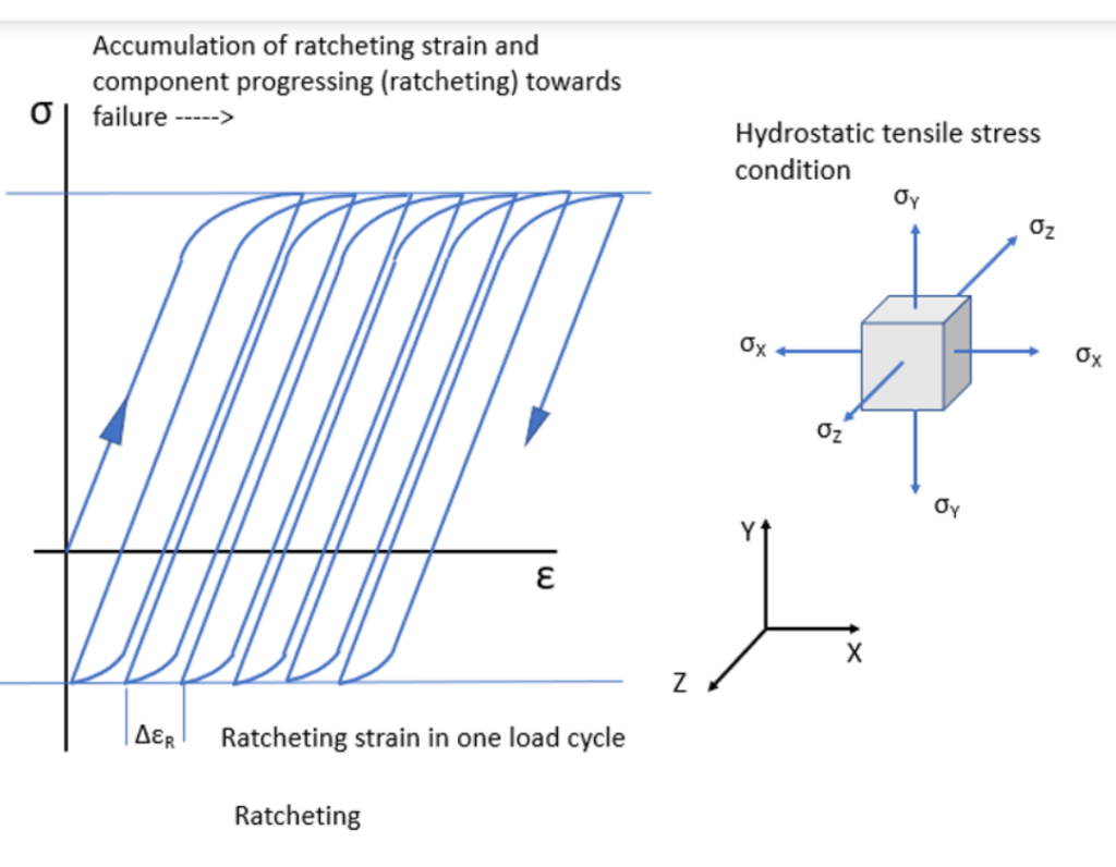
The strain-life method assumes closed, stabilized hysteresis loops. Under stress-controlled loading with a nonzero mean stress, that assumption can fail in a specific and dangerous way: each cycle deposits a small increment of plastic strain in the direction of the mean stress, and the hysteresis loops translate along the strain axis instead of closing. This is ratcheting, also called cyclic creep. The mirror-image phenomenon under strain control is mean stress relaxation, in which the loops stay put in strain but the mean stress drifts toward zero. The control mode of the loading determines which one you get:
| Control mode | Mean value present | Response |
|---|---|---|
| Strain control | Mean strain | Mean stress relaxation (benign drift toward σm = 0) |
| Stress control | Mean stress | Ratcheting (progressive strain accumulation) |
A structure that ratchets can fail by three routes: exhaustion of ductility (the accumulated strain reaches the material’s limit), geometric failure (progressive distortion, thinning, or incremental collapse renders the part nonfunctional), or accelerated fatigue, since the superimposed directional strain interacts with the cyclic damage. Damage models for combined ratcheting and fatigue often sum a Coffin-Manson term with a ductility-exhaustion term in the accumulated ratcheting strain, structurally similar to the way my dwell fatigue posts combined per-cycle rainflow damage with a time-domain damage fraction.
Shakedown Regimes and the Bree Diagram
For structures carrying a sustained primary stress (pressure, deadweight) plus a cyclic secondary stress (thermal gradients), the classical map is the Bree diagram, with primary membrane stress on one axis and cyclic thermal bending stress on the other. It partitions the response into four regimes:
- Elastic (E): no yielding anywhere; fatigue analysis proceeds elastically.
- Elastic shakedown (S): yielding in early cycles establishes a residual stress field, after which the response is purely elastic. The classical shakedown limit for a cyclic secondary stress range is \( \Delta\sigma \le 2\sigma_y \), the origin of the familiar 3Sm limit in the ASME Boiler and Pressure Vessel Code.
- Plastic shakedown (P): a closed, stable hysteresis loop with alternating plasticity every cycle; LCF governs, and the strain-life method applies directly.
- Ratcheting (R): the loop never closes; strain accumulates every cycle and the structure marches toward incremental collapse.
Design codes draw hard lines around regime R. ASME Section III (NB-3222.5) and Section VIII Division 2 provide both the elastic 3Sm screening rules and elastic-plastic ratcheting assessment procedures requiring demonstration that the accumulated strain stabilizes.
Constitutive Modeling
Capturing ratcheting in finite element analysis is notoriously demanding on the plasticity model:
- Isotropic hardening cannot ratchet at all; the yield surface simply grows and the response shakes down. Fine for monotonic analysis, wrong for this problem.
- Linear kinematic hardening (Prager) predicts closed loops and zero ratcheting, nonconservative.
- Armstrong-Frederick nonlinear kinematic hardening introduces a dynamic recovery term, \( d\boldsymbol{\alpha} = \tfrac{2}{3} C \, d\boldsymbol{\varepsilon}^p – \gamma \boldsymbol{\alpha} \, dp \), which produces ratcheting but usually overpredicts it.
- Chaboche models superpose several Armstrong-Frederick back stresses, often with a threshold on the recovery term, and remain the practical standard. Calibration against uniaxial and multiaxial ratcheting test data, not just stabilized loops, is essential; a model fit only to hysteresis loop shape can miss the ratcheting rate by an order of magnitude.
Multiaxial ratcheting, such as a pressurized pipe under cyclic bending (the classic Bree and Hassan-Kyriakides test cases), is harder still, and remains an active research area.
Practical Workflow Summary
- Obtain the load or nominal stress history; identify whether the loading is closer to stress control (force-driven) or strain control (displacement- or thermally-driven).
- Convert nominal to local notch stress-strain via Neuber or Glinka with the cyclic stress-strain curve.
- Trace hysteresis loops with material memory; rainflow counting extracts the closed loops.
- For each loop, compute strain amplitude and mean stress; apply Morrow or SWT with the strain-life constants.
- Sum damage per Miner’s rule.
- Separately screen for ratcheting whenever a sustained primary stress coexists with cyclic loading into the plastic range: Bree diagram or code rules first, Chaboche-class elastic-plastic FEA where the screening rules are not satisfied.
Closing Thoughts
The strain-life method extends fatigue analysis gracefully into the regime where stress-based methods lose their meaning, and it does so with a modest set of material constants that connect cleanly to the cyclic deformation behavior. Ratcheting is the caveat printed in bold: the method presumes closed loops, and nature does not always close them. Whenever a mean stress rides on top of plastic cycling, the analyst’s first duty is to establish which shakedown regime the structure occupies. Fatigue calculations performed in regime R are answering the wrong question.
My free ebooks on fatigue, shock, and vibration are available here: https://blog.vibrationdata.com/2025/11/27/toms-ebooks/
References
- Dowling, N.E., Mechanical Behavior of Materials, 4th Edition, Pearson, 2013.
- Bannantine, J., Comer, J., Handrock, J., Fundamentals of Metal Fatigue Analysis, Prentice Hall, 1990.
- Stephens, R.I., Fatemi, A., Stephens, R.R., Fuchs, H.O., Metal Fatigue in Engineering, 2nd Edition, Wiley, 2001.
- Manson, S.S., Behavior of Materials Under Conditions of Thermal Stress, NACA TN-2933, 1953.
- Coffin, L.F., “A Study of the Effects of Cyclic Thermal Stresses on a Ductile Metal,” Transactions of the ASME, Vol. 76, 1954.
- Neuber, H., “Theory of Stress Concentration for Shear-Strained Prismatical Bodies with Arbitrary Nonlinear Stress-Strain Law,” Journal of Applied Mechanics, Vol. 28, 1961.
- Smith, K.N., Watson, P., Topper, T.H., “A Stress-Strain Function for the Fatigue of Metals,” Journal of Materials, Vol. 5, No. 4, 1970.
- Bree, J., “Elastic-Plastic Behaviour of Thin Tubes Subjected to Internal Pressure and Intermittent High-Heat Fluxes,” Journal of Strain Analysis, Vol. 2, No. 3, 1967.
- Chaboche, J.L., “A Review of Some Plasticity and Viscoplasticity Constitutive Theories,” International Journal of Plasticity, Vol. 24, 2008.
- Hassan, T., Kyriakides, S., “Ratcheting in Cyclic Plasticity, Part I: Uniaxial Behavior,” International Journal of Plasticity, Vol. 8, 1992.
- ASME Boiler and Pressure Vessel Code, Section III and Section VIII Division 2.
📌 Related Guide & Knowledge Hub
This article is part of our comprehensive collection on Multiaxial Stress & Vibration Fatigue Analysis . Explore the full hub for methods on strain energy density, random vibration, and low-cycle fatigue.
📌 Related Earthquake Engineering Knowledge Hub
This article is featured in our main Earthquake Engineering & Structural Dynamics Hub . Visit the hub to explore related articles on shock response spectra, time history analysis, seismic equipment qualification, and structural case studies.
Looking for a deep dive on this topic? Explore our comprehensive guide and resource collection on the Residual Stress & Structural Integrity Hub.