
Figure 1. A circular laminated elastomeric bearing on a pier cap, instrumented with displacement transducers straddling the bearing and additional sensors on the pier face. The rubber cover bulges between the internal steel shim planes. Whether a lead core is buried inside is not something the exterior will tell you.
Structural health monitoring programs for bridges are built around accelerometers on the deck and the girders, because that is where the damage hypothesis lives. Cracking, section loss, corrosion, fatigue, impact damage from an over-height vehicle. The supports are usually not instrumented at all. They are inherited from the design model as an idealization, a pin at one end and a roller at the other, and the analyst carries that idealization forward into the modal interpretation without revisiting it.
That is a mistake, and the arithmetic behind why is old and completely unambiguous. The bearing is a small component. It is also the boundary condition, and the boundary condition has more leverage over the measured frequencies than anything short of gross damage in the span.
The Leverage of a Boundary Condition
For a uniform beam of length $L$, bending stiffness $EI$, and mass per unit length $\bar{m}$, the natural frequencies follow
$$ \omega_n = \lambda_n \sqrt{\frac{EI}{\bar{m}L^4}} $$
where $\lambda_n$ is a dimensionless eigenvalue set entirely by the end conditions. For the first mode, $\lambda_1=9.87$ pinned-pinned and $\lambda_1=22.37$ fixed-fixed. The ratio is 2.267. Nothing about the beam changed. Not the mass, not the section, not the material. The frequency moved by a factor of 2.27 because the ends were described differently.
Real bearings live somewhere between those two extremes, and they move along that interval over the life of the structure. The useful parameter is a nondimensional end rotational restraint
$$ \rho = \frac{k_\theta L}{EI} $$
where $k_\theta$ is the rotational stiffness the support offers against girder end rotation. Consider a reference bridge: a single 30 m span, 400 tonne deck, $EI=5.36\times10^{10}$ N-m$^2$, giving a first bending frequency of 3.50 Hz on ideal pins. It sits on four circular laminated elastomeric bearings, 450 mm bonded diameter, nine rubber layers of 8 mm each for a total rubber thickness $T_r=72$ mm, shear modulus $G=0.9$ MPa at 23 C. The vertical pressure is 6.2 MPa, which is a normal service value.
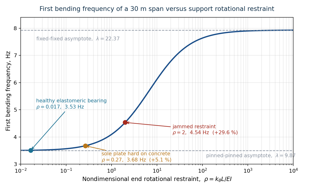
Figure 2. First bending frequency versus end rotational restraint, from a twenty-element Hermitian beam model. The model reproduces the exact eigenvalues 9.8696 and 22.3717 at the two asymptotes.
The whole transition happens over roughly three decades of $\rho$, and the steep part sits between $\rho=1$ and $\rho=30$. Everything to the left of $\rho\approx0.1$ is indistinguishable from a pin. That is the good news and it is also the trap, because it means a bearing can degrade a long way before the frequency notices, and then move quickly once it crosses into the steep region.
What a Healthy Bearing Actually Contributes
The rotational stiffness of a laminated elastomeric bearing follows from its compression modulus. For a circular bearing with shape factor $S=D/(4t)$, where $t$ is the individual layer thickness, the effective compression modulus is approximately
$$ E_c \approx 6\,G\,S^2 $$
and the rotational stiffness is $k_\theta = E_c I_b / T_r$, with $I_b=\pi D^4/64$ the bearing’s own second moment of area. For the reference bearing, $S=14.1$, $E_c=1.07$ GPa, $I_b=2.01\times10^{-3}$ m$^4$, and
$$ k_\theta = 29.9 \ \text{MN-m/rad} \qquad\Rightarrow\qquad \rho = 0.017 $$
A healthy elastomeric bearing is, to three significant figures, a pin. It raises the first bending frequency by 0.3 percent. This is exactly what the bearing was specified to do, and it is why the design idealization is defensible as long as the bearing stays healthy.
Now take the bearing away. Suppose the elastomer has been over-compressed, or has hardened and bonded, or debris has packed the gap, or the sole plate has come down onto the masonry plate. The moment path is no longer through rubber. It is steel on steel or steel on concrete, and the stiffness scale is set by the contact patch rather than by the elastomer. Treating the sole plate as a rigid circular plate on an elastic half-space of concrete, $E=30$ GPa and $\nu=0.20$,
$$ k_\theta = \frac{8GR^3}{3(1-\nu)} = 475 \ \text{MN-m/rad} \qquad\Rightarrow\qquad \rho = 0.27 $$
That is a sixteenfold jump in end rotational stiffness, and it produces a 5.1 percent rise in the first bending frequency. Nobody standing on the deck would see anything. A visual inspection at the pier might record “bearing appears in contact, no visible distress.”
| Support condition | $\rho$ | $f_1$, Hz | Change |
|---|---|---|---|
| Ideal pin, design idealization | 0 | 3.499 | reference |
| Healthy elastomeric bearing | 0.017 | 3.511 | +0.3 % |
| Sole plate hard on concrete | 0.27 | 3.679 | +5.1 % |
| Jammed or locked restraint | 2.0 | 4.536 | +29.6 % |
| Fully fixed | $\infty$ | 7.932 | +126.7 % |
The Longitudinal Mode Is a Bearing Mode
Bending is the case where the bearing is a second-order effect until it degrades. The longitudinal deck mode is the opposite. There the bearing is not a perturbation on the answer, it is the entire answer. The horizontal stiffness of a laminated bearing is
$$ K_h = \frac{G A}{T_r} $$
For the reference bearing, $K_h=1.99$ MN/m, and four of them in parallel under a 400 tonne deck give
$$ f = \frac{1}{2\pi}\sqrt{\frac{4K_h}{M}} = 0.710 \ \text{Hz} $$
Every term in that expression except the deck mass belongs to the bearing, and $G$ is strongly temperature dependent. Natural rubber stiffens as it cools, mildly down to freezing and then sharply below it as the elastomer approaches its crystallization range. Using representative stiffening factors for a natural rubber compound, referenced to 23 C:
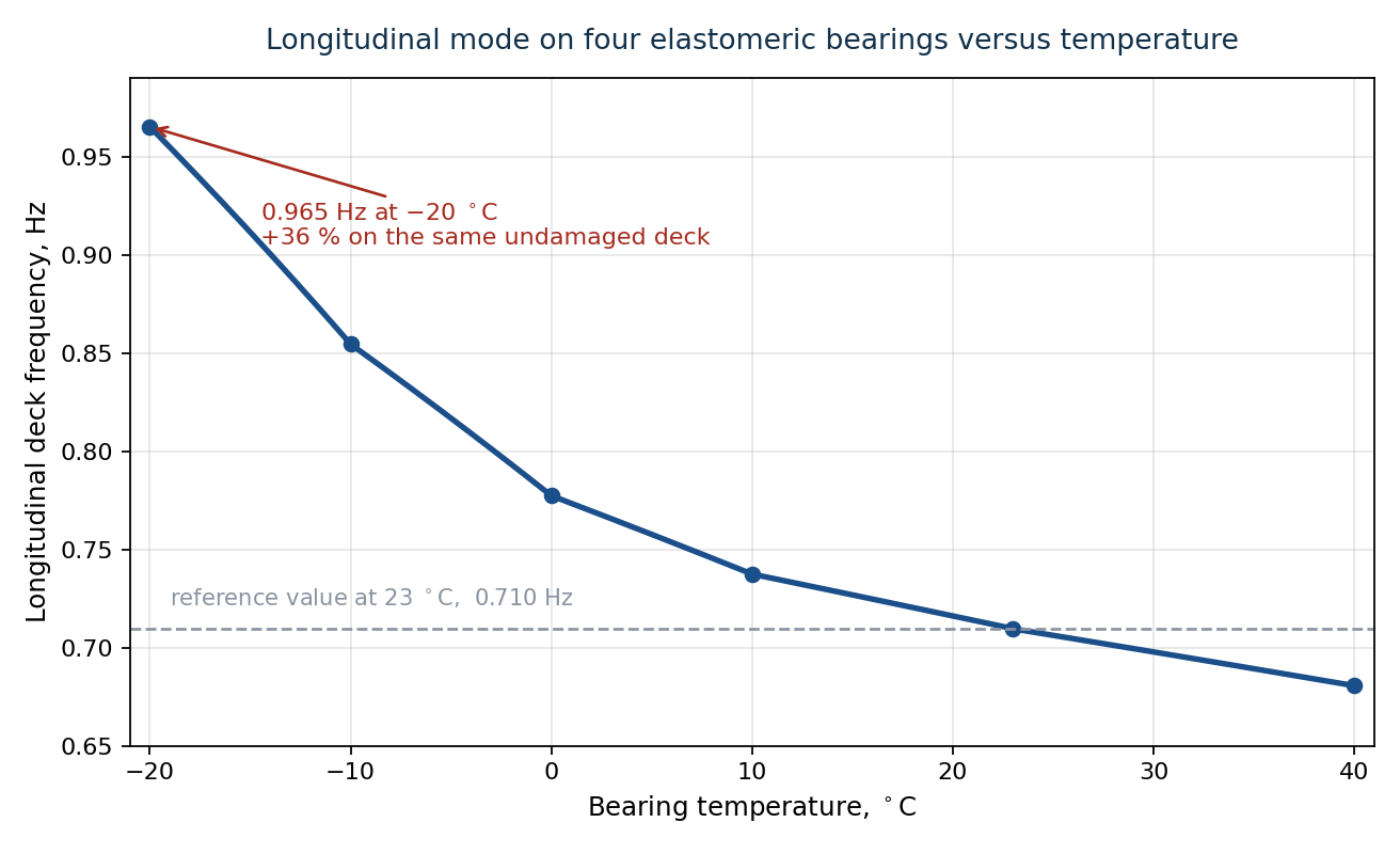
Figure 3. Longitudinal mode versus bearing temperature. Stiffening factors are representative for a natural rubber compound and are grade dependent; the actual values belong in the bearing supplier’s test report, not in a textbook.
The frequency runs from 0.681 Hz at 40 C to 0.965 Hz at $-20$ C. That is a 36 percent seasonal swing on a deck where absolutely nothing has changed. Any damage-detection scheme keying on the longitudinal mode without a temperature model is going to generate an alarm every winter and clear it every spring.
This is not a hypothetical concern. The Z24 bridge in Switzerland, monitored for a year before deliberate progressive damage and demolition, showed frequency increases below freezing that were larger than the shifts produced by the damage the experiment was designed to detect, driven by stiffening of the asphalt layer and the supports. The Alamosa Canyon bridge work at Los Alamos found roughly 5 percent variation in the first mode over a single diurnal temperature cycle. Both are environmental effects, and both would swamp a naive threshold detector.
One Seized Bearing Out of Four
Suppose a single bearing seizes longitudinally. Its load path is no longer rubber in shear. It becomes the substructure itself, and for a 1.2 m diameter pier column 5 m tall, the cantilever stiffness is
$$ K_p = \frac{3EI_p}{h^3} = 73.3 \ \text{MN/m} $$
which is nine times the combined stiffness of all four bearings. The three healthy bearings and the one seized path now total 79.3 MN/m, and the longitudinal frequency moves from 0.710 Hz to 2.240 Hz. A factor of 3.16, from one component out of four, on a deck with no damage anywhere in it.
An analyst looking only at deck accelerometers sees a mode vanish and a new one appear at three times the frequency. Every automated damage classifier ever written will flag that, and every one of them will point at the wrong part of the bridge.
The Signs Are Opposite, and That Is the Real Hazard
Damage in the span removes stiffness and lowers frequency. Restraint at the supports adds stiffness and raises it. Running both cases through the same beam model makes the comparison direct.
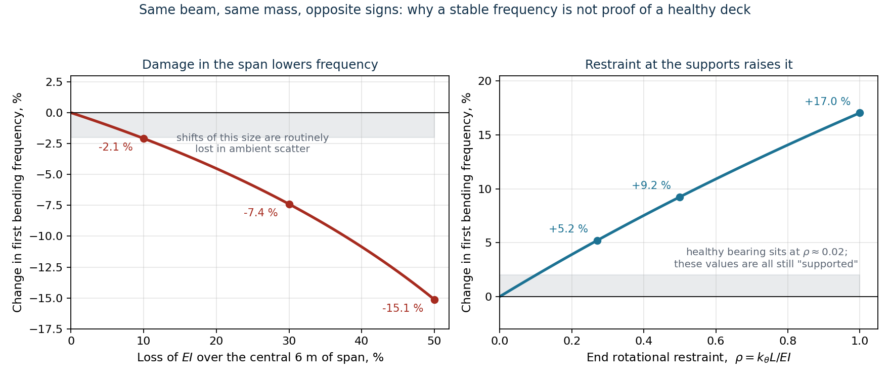
Figure 4. Left: frequency change from a uniform loss of $EI$ over the central 6 m of the span. Right: frequency change from end rotational restraint. Same beam, same mass, opposite signs.
Losing 30 percent of the bending stiffness over the central fifth of the span, which is a severe and structurally significant condition, drops the first frequency by 7.4 percent. Losing half of it drops the frequency by 15.1 percent. Meanwhile a partial end restraint at $\rho=0.5$ raises the frequency by 9.2 percent, and $\rho=1$ raises it by 17.0 percent.
The two effects are the same order of magnitude, and they have opposite signs. A bridge that is quietly losing section in the span while its bearings are quietly seizing can hold a perfectly stable first bending frequency for years. The monitoring system reports no change. Both defects are progressing. This is the failure mode that should worry anyone running a frequency-based program, and it cannot be resolved from deck accelerometers alone, because the residual carries no information about which of the two mechanisms produced it.
What to Measure at the Bearing
The instrumentation in Figure 1 is the right general idea: displacement transducers straddling the bearing, additional sensors on the pier face. What each channel buys you:
| Measurement | What it detects |
|---|---|
| Longitudinal displacement | Thermal range against design travel, run-out against a stop, progressive walking or ratcheting of the bearing |
| Lateral displacement | Transverse misalignment, skew effects, shear key engagement |
| Girder end rotation | The $\rho$ driver directly. This is the channel that separates Figure 2 from guesswork |
| Girder to support relative movement | Slip at the interface, debonding, loss of contact, uneven load sharing across bearings |
| Bearing body temperature | The $G$ correction. Note carefully: the bearing’s own temperature, not air temperature |
| Vertical displacement and uplift | Loss of contact under live load, bearing compression set, settlement of the support |
| Event-triggered capture | Step changes across a seismic event or an extreme thermal excursion, which is where bearings actually break |
The longitudinal displacement channel deserves a note, because it converts directly into an engineering acceptance quantity rather than a raw number. Shear strain in the elastomer is $\gamma=\Delta/T_r$. For the reference bearing, $T_r=72$ mm, so a design limit of $\gamma=0.7$ for the slow thermal component corresponds to 50 mm of travel. A 30 m steel deck with the thermal center at midspan and a 60 C annual range moves about $\pm11$ mm at each end, giving $\gamma\approx0.15$. Comfortable. If that reading starts drifting toward the limit over successive years, the bearing is walking, and you know it from a single displacement channel long before it reaches a stop and starts transferring moment.
Two Cautions
First, a temperature channel does not cleanly isolate the bearing’s contribution. Temperature simultaneously changes the elastomer shear modulus, the asphalt and deck stiffness, expansion joint engagement, and in some structures the soil around the abutments. All of those move the frequency, some of them with hysteresis, and they are correlated with each other because they share a driver. Measuring bearing temperature is necessary. It is not sufficient, and a single-variable regression against temperature will leave structure in the residual that has nothing to do with damage.
Second, the bearing’s own body temperature lags air temperature by hours because of its thermal mass. Regressing modal frequency against ambient air temperature therefore produces a hysteresis loop rather than a curve, and the loop width is mistaken for scatter. Put the sensor in or on the bearing.
Which leads to the part that most programs underestimate. Before a modal change means anything, you need enough baseline to have seen the full seasonal envelope, including the cold tail where the elastomer stiffening is steepest. The first year of data is calibration, not detection. Deploying a threshold detector in month two and acting on its output is not monitoring, it is generating false positives with instrumentation.
References and Further Reading
Peeters, B. and De Roeck, G., “One-year monitoring of the Z24-Bridge: environmental effects versus damage events,” Earthquake Engineering and Structural Dynamics, Vol. 30, 2001.
Farrar, C. R., et al., “Variability of modal parameters measured on the Alamosa Canyon Bridge,” Los Alamos National Laboratory.
Sorensen, C. J. and Kelly, J. M., Mechanics of Rubber Bearings for Seismic and Vibration Isolation, Wiley.
AASHTO LRFD Bridge Design Specifications, Section 14, Joints and Bearings.
EN 1337-3, Structural bearings, Part 3: Elastomeric bearings.
Related Vibrationdata material on modal parameters, boundary conditions, and structural dynamics is collected in the free ebook set at https://blog.vibrationdata.com/2025/11/27/toms-ebooks/