Every introductory vibration course begins by drawing a mass on a spring and declaring that the spring has stiffness but no mass. That assumption is the reason the single-degree-of-freedom system has exactly one natural frequency instead of infinitely many. It is an excellent assumption almost all of the time. It fails in a specific and expensive way when the spring is asked to control motion at a frequency approaching its own internal resonances.
That failure is called spring surge. A real spring is a slender elastic body with distributed mass, and it will carry longitudinal waves along its axis exactly as a rod does. When those waves reflect from the spring’s ends and resonate, the coils no longer move together as a unit. Some coils accelerate while others decelerate. The spring stops behaving as a stiffness element and starts behaving as a structure with its own dynamics.
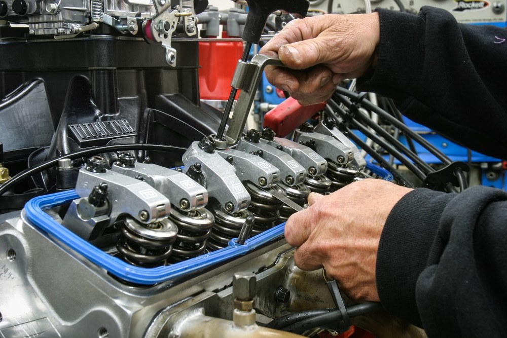
Figure 1. Valve springs and lifters. The valve spring is the classic surge victim because the camshaft feeds it a periodic input rich in harmonics.
The Spring is a Rod
Consider a coil spring of free length $L$, total stiffness $k$, and total mass $m$, with mass per unit length $\rho_L = m/L$. Model it as a uniform rod in longitudinal vibration. The governing equation is the one-dimensional wave equation, and the wave speed is
$$c = \sqrt{E/\rho} = L\sqrt{k/m}$$
The second form follows from recognizing that an equivalent rod of the same stiffness satisfies $EA = kL$, while $\rho A = m/L$. The natural frequencies then follow the standard longitudinal rod results, with the boundary conditions determining the coefficient.
| Configuration | Natural Frequencies | Mode Shapes |
|---|---|---|
| Fixed-Free | $f_n = \dfrac{(2n-1)}{4}\sqrt{\dfrac{k}{m}}$ | $U(x) = \sin\!\left(\dfrac{(2n-1)\pi x}{2L}\right)$ |
| Free-Free | $f_n = \dfrac{n}{2}\sqrt{\dfrac{k}{m}}$ | $U(x) = \cos\!\left(\dfrac{n\pi x}{L}\right)$ |
| Fixed-Fixed | $f_n = \dfrac{n}{2}\sqrt{\dfrac{k}{m}}$ | $U(x) = \sin\!\left(\dfrac{n\pi x}{L}\right)$ |
with $n = 1, 2, 3, \ldots$ Note that the length cancels out of the frequency expressions. The surge frequencies depend only on the ratio of total stiffness to total mass, which is convenient because both are quantities a spring vendor already publishes.
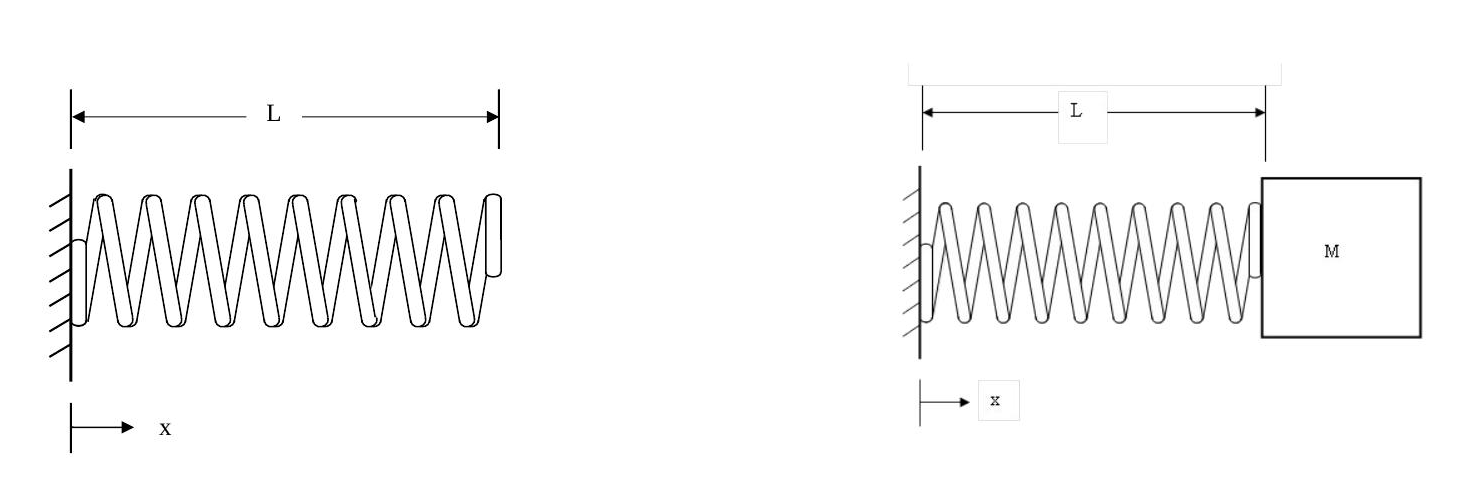
Figure 2. The two models that cover most practical cases. Left: a spring fixed at one end with a free end. Right: the same spring carrying an end mass M.
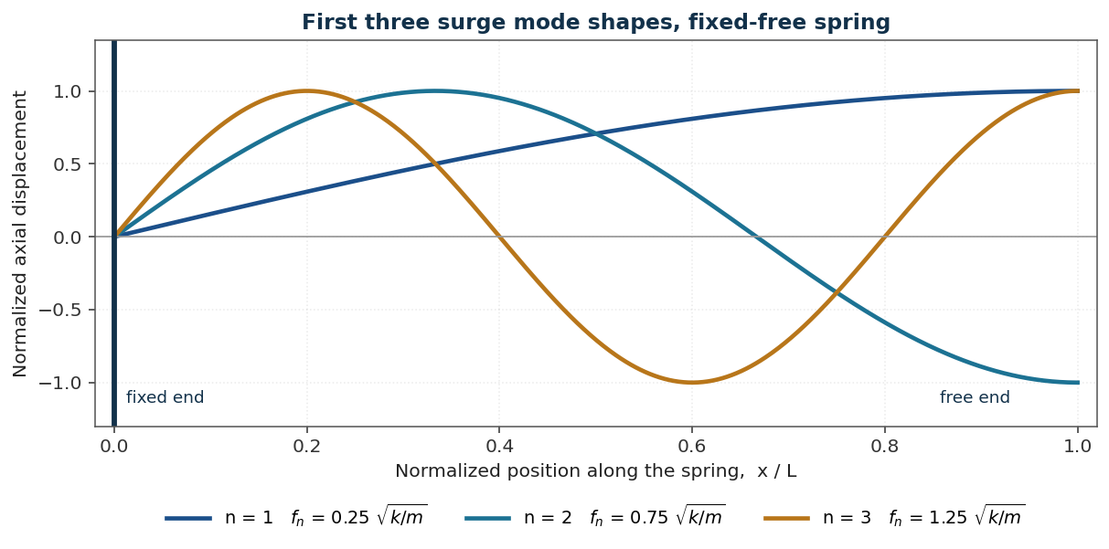
Figure 3. Surge mode shapes. In the second mode there is an interior node where one coil group is moving up while another moves down. The coils on either side of that node are being compressed toward each other, which is how surge produces coil clash and local stress far above the nominal working stress.
A Factor That Catches People
The fixed-free fundamental is $f_1 = 0.25\sqrt{k/m}$ in Hz. Everyone who has done vibration work has the expression $\sqrt{k/m}$ wired to $\omega_n$ in rad/sec, and the reflex is to divide by $2\pi$. That reflex is wrong here. The surge coefficient is $1/4$, not $1/(2\pi)$, and the two differ by
$$\frac{1/4}{1/(2\pi)} = \frac{\pi}{2} = 1.5708$$
The units work out because $\sqrt{k/m}$ appears here through $c/L$, a genuine reciprocal-seconds quantity, rather than through the SDOF circular frequency. Anyone who divides by $2\pi$ out of habit will underestimate the first surge frequency by 36 percent and conclude that a perfectly good spring is unsafe.
Sanity check. If a spring is idealized as massless and given the spring’s own mass as a lumped end mass, the resulting SDOF frequency is $\frac{1}{2\pi}\sqrt{k/m}$. The true first surge frequency is $\pi/2$ times higher. Different model, different answer, and the wave model is the correct one.
The Spring With an End Mass
Most real installations put something on the end of the spring: a valve and retainer, a compressor head, a piece of machinery. Let $M$ be the end mass and define the mass ratio
$$\mu = \frac{M}{m}$$
The eigenvalue problem is no longer trigonometric in closed form. Applying Newton’s law to the end mass, with the internal rod force $EA\,u'(L)$, gives the transcendental characteristic equation
$$\beta L\,\tan(\beta L) = \frac{m}{M} = \frac{1}{\mu}, \qquad f_n = \frac{\beta_n L}{2\pi}\sqrt{\frac{k}{m}}$$
The two limiting cases are worth committing to memory. As $\mu \to 0$ the roots approach $(2n-1)\pi/2$, recovering the fixed-free result. As $\mu \to \infty$ the roots approach $(n-1)\pi$, so the higher modes recover the fixed-fixed result while the first root collapses toward zero and becomes the familiar rigid-body isolation mode. In other words, a heavy end mass turns a free end into a fixed end as far as the surge waves are concerned, because the mass has too much inertia to move at those frequencies.
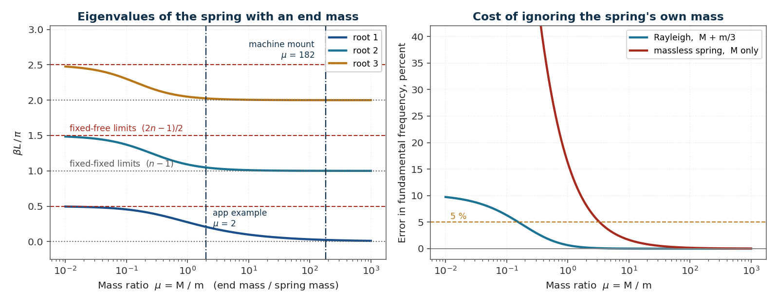
Figure 4. Left: the first three roots migrate from the fixed-free limits to the fixed-fixed limits as the end mass grows. Right: the error committed by the two common shortcuts for the fundamental frequency.
For the fundamental mode alone there is a well-known Rayleigh approximation that adds one third of the spring mass to the end mass
$$f_1 \approx \frac{1}{2\pi}\sqrt{\frac{k}{M+0.33\,m}}$$
The right panel of Figure 4 shows why this approximation has survived for a century. It stays within 1 percent for $\mu>0.76$ and within 5 percent all the way down to $\mu\approx0.16$. By contrast, simply ignoring the spring mass altogether costs 5 percent at $\mu=3.3$, does not reach 1 percent until $\mu=17$, and grows without bound as the spring gets heavier. But note the limitation that matters most: the one-third rule gives only the fundamental. It says nothing whatsoever about the surge modes, which is precisely the information a high-speed application needs.
Worked Example
Take $k = 10{,}000$ lbf/in and a spring mass of 1 lbm, which is $1/386.09 = 0.002591$ lbf-sec$^2$/in. Then $\sqrt{k/m} = 1964.9$ sec$^{-1}$.
| Case | Mode 1 | Mode 2 | Mode 3 |
|---|---|---|---|
| Fixed-free, no end mass | 491.2 Hz | 1473.7 Hz | 2456.1 Hz |
| Fixed-fixed or free-free | 982.5 Hz | 1964.9 Hz | 2947.4 Hz |
| Fixed with 2 lbm end mass, $\mu = 2$ | 204.3 Hz | 1029.6 Hz | 1989.4 Hz |
For the third case the roots are $\beta L = 0.6533$, $3.2923$, and $6.3616$. The Rayleigh one-third approximation gives 204.7 Hz for the fundamental, high by 0.21 percent. Neglecting the spring mass entirely gives 221.1 Hz, high by 8.2 percent. And the first true surge mode sits at 1029.6 Hz, a frequency that neither shortcut predicts at all.
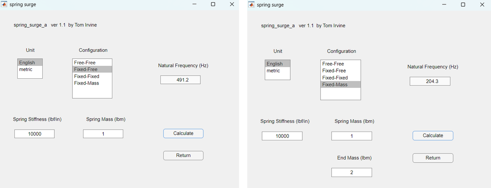
Figure 5. The spring surge function in the Vibrationdata MATLAB GUI package, reached through Structural Dynamics > Spring-Mass Systems > Single > Spring Surge. It covers free-free, fixed-free, fixed-fixed, and fixed-mass, in English or metric units, and solves the transcendental equation for the fixed-mass case rather than using the one-third approximation.
Automotive Valve Springs
The valve spring is the canonical surge problem, and racing engines live closest to the edge. Surge is among the most common limiters in high-speed valvetrains. The first symptom is usually a localized dip in the dyno power curve at a particular engine speed, which is often misdiagnosed as a fuel or ignition fault because it appears and disappears with rpm rather than with load.
The forcing function is the harmonic content of the cam lift profile. A cam lobe is a periodic, decidedly non-sinusoidal displacement input, so its Fourier series contains energy at every integer multiple of camshaft rotation frequency. The low-order harmonics carry the largest amplitudes and the content falls off rapidly with order. This gives the classical design rule:
Design rule of thumb. The fundamental surge frequency should be at least 8 to 13 times the camshaft rotation frequency. At 8000 rpm crankshaft, the camshaft turns at 4000 rpm, which is 66.7 Hz. The eighth harmonic is 533 Hz, and the first surge mode must clear it.
Which boundary condition applies?
Spring catalogs and the classical valve spring literature quote the fixed-fixed value, $f_1 = 0.5\sqrt{k/m}$, and there is a good physical reason. While the follower is in contact with the cam, both ends of the spring are kinematically driven. The seat end is fixed to the head and the retainer end is driven by the cam through the valve. Neither end is free to respond to the surge wave, so both are effectively fixed. The classical closed-form version of that result for a steel helical spring is
$$f_1 = \frac{d}{2\pi D^2 N}\sqrt{\frac{G}{2\rho}} \;\approx\; \frac{13{,}900\,d}{N D^2}\ \text{Hz}$$
with $d$ the wire diameter and $D$ the mean coil diameter in inches, and $N$ the number of active coils. This follows directly from substituting $k = Gd^4/(8D^3N)$ and $m = \rho\,\pi^2 d^2 D N/4$ into $f_1 = 0.5\sqrt{k/m}$.
Once the follower separates from the cam, which is the onset of valve float, the boundary condition changes to fixed-mass with the retainer, keepers, and valve as $M$. That mode is much lower, and for a typical racing spring it lands in the low hundreds of Hz. It is not a surge mode in the usual sense, but it is the mode that governs valve bounce and seat impact.
A racing spring
Take a single racing valve spring with wire diameter $d = 0.185$ in, mean coil diameter $D = 1.05$ in, and 4 active coils, in steel with $G = 11.5\times10^6$ psi and 0.283 lbm/in$^3$.
| Quantity | Value |
|---|---|
| Rate, $k = Gd^4/(8D^3N)$ | 363.6 lbf/in |
| Active-coil mass | 0.1004 lbm |
| $\sqrt{k/m}$ | 1182.7 sec$^{-1}$ |
| Surge modes, fixed-fixed | 591, 1183, 1774 Hz |
| Order at 8000 rpm crank | 8.9 |
The classical formula gives 583 Hz against the 591 Hz computed from $k$ and $m$ directly, the small difference coming from the rounded 13,900 constant. At 8000 rpm the first surge mode is riding at order 8.9, just inside the acceptable band and uncomfortably close to the ninth harmonic at 600 Hz. Figure 6 shows how quickly that margin evaporates.
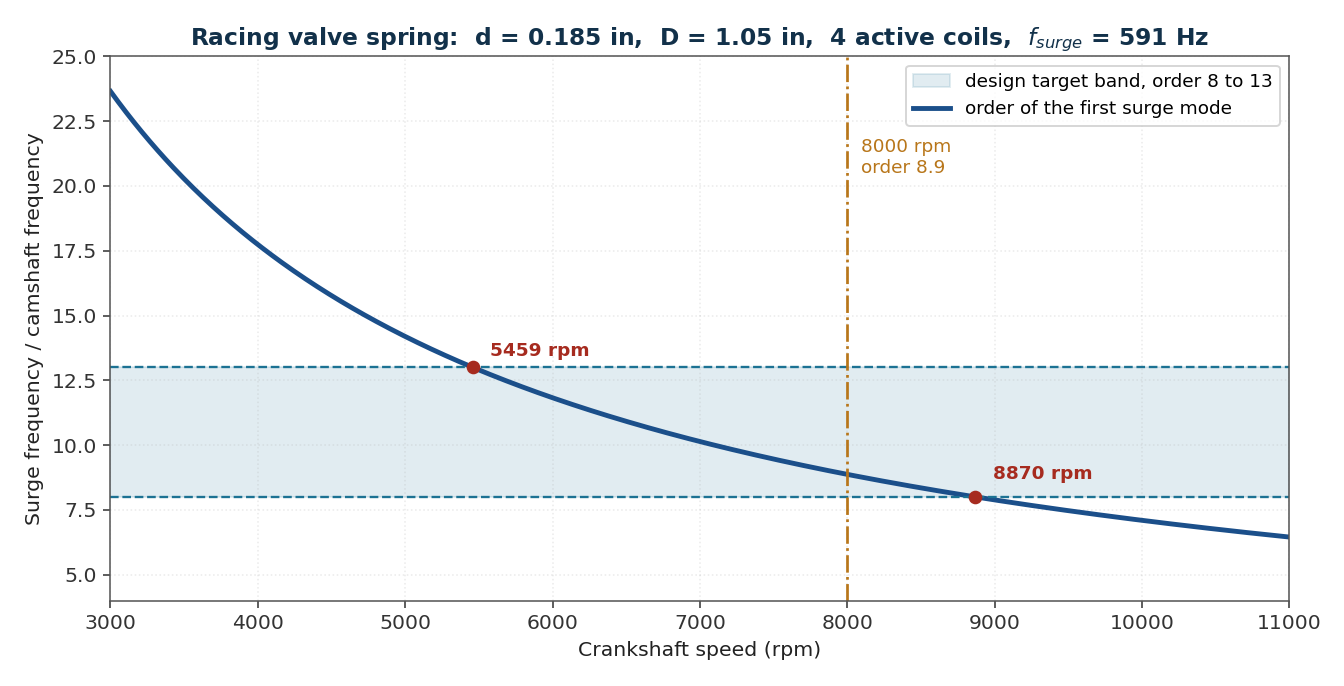
Figure 6. The surge frequency is fixed by the spring; the excitation order is fixed by engine speed. The margin runs out at 8870 rpm for this spring, and everything above that line is territory where the cam is feeding energy directly into a surge mode.
Note that the order ratio is inversely proportional to rpm, so it degrades fastest exactly where the engine is making the most power. Note also that the surge frequency scales as $d/(ND^2)$. Adding a single active coil to this spring drops the surge frequency by 20 percent and the order at 8000 rpm from 8.9 to 7.1, below the design band. That is why valve springs are short and stiff, and why the temptation to add coils for a softer ride is resisted so firmly.
Consequences and countermeasures
The consequences escalate with speed. First comes the power dip. Then valve float and seat bounce, as the spring can no longer deliver the force the cam profile demands. Then coil clash, spring fatigue fracture, and eventually a dropped valve, which is generally the end of the engine.
The countermeasures fall into three families. Detune the spring: raise $d$, lower $D$, remove active coils, or shim closer to coil bind so the working portion of the spring is shorter and stiffer. Break the resonance: interference-fit dual or triple springs so that the inner and outer springs have different surge frequencies and rub against each other, and use variable-pitch or beehive geometry so that no single uniform section can support a clean standing wave. Add damping: flat-ribbon friction dampers nested inside the spring, which is the only practical way to add loss to a steel spring whose material damping is negligible.
Two case histories
| Case | Problem and fix |
|---|---|
| Mercedes-Benz W196 Formula One, 1954 to 1955 |
Development testing repeated a defect of the 1930s Silver Arrows: valve gear trouble above 8000 rpm and fragile springs. The fix was desmodromic valve gear, in which cams and rockers close the valve as well as open it, deleting the spring altogether. The result was 290 hp at 8500 rpm and nine wins in twelve races. |
| Renault Formula One Pneumatic valve springs, 1986 |
Steel springs capped engine speed near 12,000 rpm through resonance and fatigue, limiting the 1.5 liter turbo engines. The fix was nitrogen-charged pneumatic springs replacing the steel coils, debuted in the Lotus 98T. The approach is universal in Formula One and MotoGP today, enabling 15,000+ rpm. |
These are two classical resonance strategies applied to the same problem: remove the resonant element, or replace it with one whose distributed mass is negligible. A gas column has stiffness with essentially no inertia at these frequencies, which is exactly the massless spring that textbooks assume and steel refuses to be.
Spring Surge in Isolation Mounts
The second place surge shows up, and the one more likely to affect a structural dynamicist, is the steel coil isolator under a piece of machinery. Here the effect is not fatigue fracture; it is a quiet loss of the isolation the mount was purchased to provide.
Solving the base-excited rod carrying an end mass gives an exact transmissibility, where $\beta L=\omega\sqrt{m/k}$ and $\mu=M/m$
$$T = \frac{1}{\cos(\beta L)-\mu\,\beta L \sin(\beta L)}$$
Expand for small $\beta L$ and this reduces to $T = 1/(1-(\omega/\omega_0)^2)$, the textbook massless result, confirming the formula. The poles are the fixed-mass natural frequencies. Consider a mount with a 12 mm wire, 75 mm mean coil diameter, and 6 active coils, carrying 229 kg.
| Quantity | Value |
|---|---|
| Stiffness | 81.2 kN/m |
| Coil mass | 1.26 kg |
| Static deflection | 27.7 mm |
| Isolation frequency $f_0$ | 3.00 Hz |
| Mass ratio $\mu$ | 182 |
| Surge modes | 127.2, 254.4, 381.6 Hz |
Because $\mu$ is large, the surge frequencies follow the fixed-fixed limit, and they can be written in a form worth remembering
$$f_{surge,n} \approx n\,\pi\sqrt{\mu}\;f_0$$
The first surge mode is $\pi\sqrt{182} = 42.4$ times the isolation frequency. That number is the whole design problem in one place: the ratio of the first surge frequency to the isolation frequency is fixed by the square root of the mass ratio, and there is no way to push the surge up without either making the mount heavier to carry or the spring lighter.
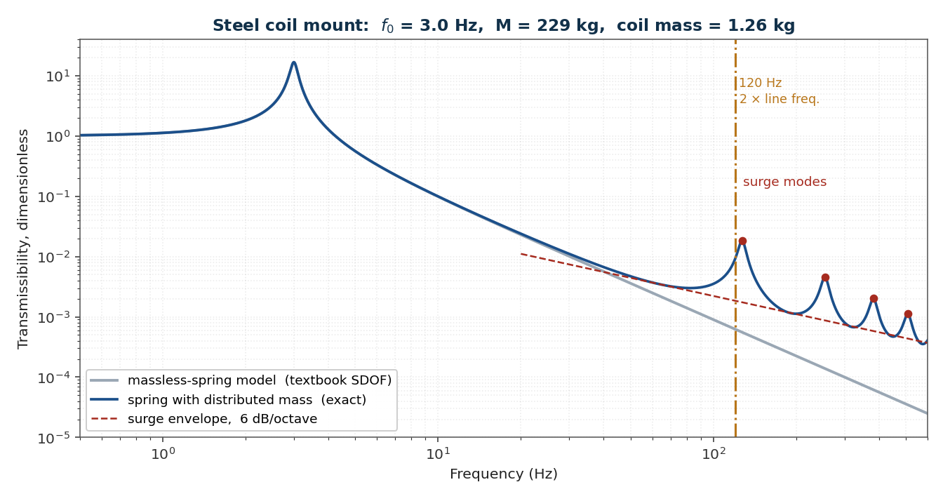
Figure 7. Exact transmissibility of the steel coil mount against the massless-spring prediction, both with 6 percent loss factor. The two agree perfectly through the isolation region and diverge above roughly 40 Hz.
Two features of Figure 7 deserve attention. The first is the obvious one: there are resonant peaks at the surge frequencies where the massless model predicts monotonic rolloff. At 127.2 Hz the exact transmissibility is 0.0185 against a predicted 0.00056, a factor of 33, or 30 dB.
The second is subtler and, in most installations, more damaging. Between the surge peaks the exact curve does not return to the massless curve. Its floor follows an envelope of $1/(\mu\,\beta L)$, which decays as $1/f$. A real steel spring isolates at 6 dB per octave in the mean, not the 12 dB per octave the SDOF model promises. The error therefore accumulates with frequency whether or not a surge mode happens to line up with a forcing frequency.
For this mount, twice line frequency at 120 Hz is a permanent feature of any motor-driven machine. The massless model predicts a transmissibility of 0.00062, or 99.94 percent isolation. The exact model gives 0.0091, or 99.09 percent. That is 15 times the transmitted motion, and it is the difference between a specification that is met and one that is missed. The mount was designed by placing $f_0$ a factor of 40 below 120 Hz, and that arithmetic was correct; the model was not.
Why the surge wave is so slow
A helical spring is a torsion bar wound into a helix, and the surge wave is really a torsional wave travelling along the wire. The helix geometry converts wire twist into axial coil motion with a large mechanical advantage, so the effective axial wave speed $c = L\sqrt{k/m}$ lands in the tens of metres per second, three orders of magnitude below the 3200 m/sec shear wave speed of the steel itself. The exact relationship between the axial surge frequency and the half-wave frequency of a straight wire of the same length is
$$\frac{f_{surge}}{f_{wire}} = \frac{d}{\sqrt{2}\,D}$$
For the mount above, $d/(\sqrt{2}D) = 0.113$, and 1124 Hz becomes 127 Hz. This is the reason surge frequencies are low enough to matter. If a coil spring behaved acoustically like a steel bar, surge would be an ultrasonic curiosity rather than a design constraint.
Practical mitigation for mounts
- Put an elastomeric pad in series with the steel spring. This is why quality spring isolators ship with a neoprene or cork pad under the base plate, and it is not a shipping accessory. The pad has high internal damping and no comparable internal resonance in the audio range, so it breaks the surge transmission path.
- Check the surge frequencies against the machine’s actual forcing set. Shaft speed, blade or vane pass, gear mesh, line frequency and twice line frequency, and rotor bar pass. The surge frequencies are computable from the vendor’s published rate and spring weight in about a minute.
- Do not accept the SDOF rolloff for structure-borne noise predictions. Above roughly ten times the isolation frequency, use the exact expression or accept that the prediction is optimistic.
- Watch springs with a high mass ratio between mount and spring. Counterintuitively, a small mass ratio pushes the surge frequencies up relative to $\sqrt{k/m}$, but it also lowers $f_0$ relative to the surge. The ratio $\pi\sqrt{\mu}$ is what governs.
Where Else Surge Appears
| Application | Excitation Source | Effect of Surge | Mitigation |
|---|---|---|---|
| Engine valve springs | Camshaft rotation | Valve float, failure | Dual springs, damping, higher spring stiffness, nitrogen-charged pneumatic springs |
| Compressors and pumps | Rotating and reciprocating motion | Spring fatigue | Higher spring stiffness, damping |
| Clutch and flywheel dampers | Engine torque pulsation | Rattling, torsional vibration | Tuned dampers, progressive stiffness |
| Railcar buffers | Train coupling | Ineffective shock absorption | Friction elements, hydraulic buffers |
| Robotic actuators | High-speed mechanical load | Inaccuracy, spring failure | Short and stiff springs, tuned resonance |
| Equipment isolation mounts | Line frequency, blade pass, gear mesh | Loss of high-frequency isolation, structure-borne noise | Elastomeric pad in series, exact transmissibility check |
| Relief and control valves | Flow pulsation, acoustic modes | Chatter, seat wear | Stiffer springs, damping, pulsation control |
A Note on Stress
Once a surge mode is excited, the coils near an interior node experience relative displacement that the static rate calculation does not capture. The relevant stress is a travelling shear wave in the wire, and the classical relationship $\tau = \rho\, c_s\, v$ applies, with $c_s$ the shear wave speed in the material and $v$ the particle velocity in the wire. The practical consequence is that a modest surge amplitude can add a large alternating shear stress on top of the working stress, because the coefficient $\rho c_s$ for steel is large. The wire in a surging spring is being fatigued at a frequency hundreds of times higher than the shaft speed, so cycles accumulate very quickly. This is the mechanism behind both the valve spring fracture and the fatigue entry in the compressor row of the table above. The helix geometry means this should be treated as an order-of-magnitude estimate rather than a design stress, but it explains why surge failures arrive so much faster than the nominal duty cycle suggests.
Summary
- A spring has mass. Above roughly ten times the fundamental of the system it controls, that mass governs the behavior and the massless idealization stops being useful.
- Surge frequencies depend only on $\sqrt{k/m}$ and the boundary conditions. The coefficient is $(2n-1)/4$ fixed-free and $n/2$ for both fixed-fixed and free-free, and the result is in Hz without dividing by $2\pi$.
- With an end mass, solve $\beta L \tan(\beta L) = m/M$. The Rayleigh $M+m/3$ rule handles the fundamental well but tells you nothing about the surge modes.
- In valve trains, keep the surge frequency 8 to 13 times the camshaft frequency at redline. Dual springs, variable pitch, beehive geometry, friction dampers, and pneumatic springs are the standard answers.
- In isolation mounts, the first surge frequency is about $\pi\sqrt{M/m}$ times the isolation frequency, and the isolation floor rolls off at 6 dB per octave rather than 12. Put an elastomeric pad in series and check the surge frequencies against the machine’s forcing set.
References
- T. Irvine, Longitudinal Natural Frequencies of Rods and Response to Initial Conditions, Rev K, Vibrationdata.
- T. Irvine, Structural Dynamics Special Topics, Rev F, Vibrationdata, 2026.
- A. M. Wahl, Mechanical Springs, 2nd edition, McGraw-Hill, 1963.
- SAE AE-21, Spring Design Manual, 2nd edition, Society of Automotive Engineers, 1996.
- W. T. Thomson and M. D. Dahleh, Theory of Vibration with Applications, 5th edition, Prentice Hall, 1998.
- C. M. Harris and A. G. Piersol, editors, Harris’ Shock and Vibration Handbook, 5th edition, McGraw-Hill, 2002.
- Vibrationdata MATLAB stand-alone executable GUI package, blog.vibrationdata.com/2022/09/28/vibrationdata-matlab-stand-alone-executable-gui-package/
Free ebooks on shock, vibration, fatigue, and acoustics are available at blog.vibrationdata.com/2025/11/27/toms-ebooks/