The Barrett scaling law is one of the oldest tools in the launch vehicle random vibration toolbox, and it is still one of the most used. It answers a question that comes up on every new program before a single accelerometer has been mounted: I have flight data from a previous vehicle, and I have an acoustic prediction for the new one. What vibration level should I write into the component specification?
The method extrapolates a measured reference environment to a new structure using three ratios: the acoustic pressure, the mass per unit area of the backup structure, and the mass loading of any component riding on that structure.
$$ G_N(f) = G_R(f) \left[ \frac{P_N(f)}{P_R(f)} \right]^{2} \left[ \frac{M_R}{M_N} \right]^{n} \left[ \frac{W_N}{W_N + W_C} \right] $$| f | Frequency (Hz) |
| GN(f) | New vehicle acceleration power spectral density, G²/Hz |
| GR(f) | Reference vehicle acceleration power spectral density, G²/Hz |
| PN(f) | New vehicle measured or predicted acoustic pressure, RMS |
| PR(f) | Reference vehicle acoustic pressure, RMS |
| MN | Mass per unit area of the new structure |
| MR | Mass per unit area of the reference structure |
| WN | Weight of the new structure backup area |
| WC | Weight of the component mounted on the new structure backup area |
| n | Mass ratio exponent — the subject of this post |
The pressure ratio exponent is not controversial. Power spectral density is a mean square quantity, so it scales with the square of pressure by definition. The mass loading term is not controversial either. The exponent on the mass per unit area ratio, however, has a history. Barrett’s original derivation gives n = 2. Every practical application of the method that I am aware of uses n = 1. This post is about why.
Where the Squared Exponent Comes From
Consider a rigid patch of skin of area A and mass m, driven by a fluctuating pressure p(t). Newton’s second law gives the acceleration directly.
$$ \ddot{x}(t) = \frac{A\, p(t)}{m} \qquad \Rightarrow \qquad G_{\ddot{x}}(f) = \left( \frac{A}{m} \right)^{2} G_p(f) $$Double the mass and the acceleration halves, so the acceleration PSD drops by a factor of four. The same result falls out of a single-mode treatment. For a mode with generalized mass Mn, resonant frequency fn, and amplification factor Q, driven by a generalized force PSD SF that is flat near resonance, the mean square acceleration is
$$ \left\langle \ddot{x}^{2} \right\rangle = \frac{\pi}{2}\, f_n\, Q\, \frac{S_F(f_n)}{M_n^{2}} $$With a generalized force built from a pressure field acting over the panel, $S_F = A^2 j_n^2(f)\, S_p(f)$, where $j_n^2$ is the joint acceptance, and with generalized mass $M_n \approx \tfrac{1}{2}\rho_s A$ for a mass per unit area $\rho_s$, this becomes
$$ \left\langle \ddot{x}^{2} \right\rangle \;\propto\; \frac{j_n^{2}\, S_p}{\rho_s^{2}} $$So the squared exponent is not sloppy work. It is exactly correct for a force-controlled response: one in which the excitation delivers a prescribed force, and the structure’s only job is to divide that force by its mass.
Why the Force-Controlled Picture Fails
When a skin section gets heavier per unit area, several things change at once, and they do not all push the response in the same direction.
Acoustic coupling improves. Increasing the thickness raises the bending wave speed, which lowers the critical, or coincidence, frequency.
$$ f_c \;=\; \frac{c_0^{2}}{1.8\, c_L\, h} $$Below coincidence, a panel is a poor acoustic radiator and, by reciprocity, a poor acoustic absorber. Pushing $f_c$ down means that at any given analysis frequency the heavier panel is closer to, or above, coincidence. Its wavenumber is better matched to the pressure field. Joint acceptance and radiation efficiency both rise. The heavier panel therefore does not see the same generalized force. It sees more of the field.
Modal density drops. The resonant mode count per unit bandwidth for a flat plate is independent of frequency and inversely proportional to thickness.
$$ n(f) \;=\; \frac{\sqrt{3}\, A}{h\, c_L} $$Fewer modes in a band means fewer resonant contributions to the band-limited response. This one pushes the other way, toward a steeper mass dependence than the square.
Damping is not constant. Heavier structural configurations in a real vehicle are not simply thicker sheets. They carry more frames, more stringers, more fasteners, more brackets, and more attached hardware. Joint damping and mass-loading damping both tend to rise with structural weight. Higher loss factor means lower resonant response, which again is not captured by any exponent on mass alone.
Mass per unit area is not an independent variable. In a databank assembled from flight measurements, mass per unit area is entangled with structural configuration, with location on the vehicle, with the character of the local pressure field, and with the boundary conditions at the panel edges. Fitting a single exponent through that scatter is a regression, not a derivation.
The honest summary is that the mass exponent is an empirical exponent that has to absorb all of these competing effects. Newton’s second law describes exactly one of them.
The Power Balance Gives an Exponent of One
There is a second idealization, and it is the more appropriate one for a lightly damped structure with many resonant modes in the analysis band. Instead of a force balance, write a power balance. In steady state the power delivered by the acoustic field equals the power dissipated by structural damping.
$$ \Pi_{\mathrm{in}} \;=\; \omega\, \eta\, M \left\langle v^{2} \right\rangle \;=\; \omega\, \eta\, \rho_s A \left\langle v^{2} \right\rangle $$Solve for the space-averaged mean square velocity, then convert to acceleration.
$$ \left\langle v^{2} \right\rangle \;=\; \frac{\Pi_{\mathrm{in}}}{\omega\, \eta\, \rho_s A} \qquad \Rightarrow \qquad \left\langle a^{2} \right\rangle \;=\; \omega^{2} \left\langle v^{2} \right\rangle \;=\; \frac{\omega\, \Pi_{\mathrm{in}}}{\eta\, \rho_s A} $$If the acoustic field delivers roughly the same power per unit area regardless of how heavy the panel is — which is what the competing effects listed above tend to produce, since improving coupling partially offsets falling modal density — then the acceleration PSD varies as the inverse first power of mass per unit area. That is the exponent used in practice.
The Energy Interpretation
The first-power law has a compact physical statement. Rearrange it as
$$ \rho_{s,N} \left\langle v_N^{2} \right\rangle \;=\; \rho_{s,R} \left\langle v_R^{2} \right\rangle $$The kinetic energy per unit area is preserved between the reference structure and the new one. The acoustic field deposits a certain amount of vibrational energy into each square foot of skin, and how that energy is split between velocity and mass is the structure’s business, not the field’s. The squared law says something quite different: it says the impulse per unit area is preserved, and that the vibrational energy per unit area falls off as $1/\rho_s$. The field would have to become less effective at driving the structure in exact proportion to how heavy the structure is, with no compensating improvement in coupling. That is not what happens.
There is a useful corollary for anyone who works in stress-velocity terms. Using the elementary relationship between dynamic bending stress and modal velocity,
$$ \sigma \;=\; \rho\, c\, V \qquad \Rightarrow \qquad \frac{\sigma_N}{\sigma_R} \;=\; \frac{V_N}{V_R} \;=\; \sqrt{ \frac{\rho_{s,R}}{\rho_{s,N}} } $$Under the first-power law, a 4:1 increase in mass per unit area cuts the dynamic stress in half. Under the squared law it would cut it by a factor of four. The first result is much closer to what acoustic test data on skin panels actually show, and it is a good reminder that thickening a skin buys you less fatigue margin against an acoustic environment than a naive force argument suggests.
Barrett’s Own Mass Loading Term Is Already First Power
There is an internal consistency argument hiding in the equation itself. Look at the last bracket.
$$ \left[ \frac{W_N}{W_N + W_C} \right]^{1} $$This is the mass loading attenuation: hang a component on a panel and the panel responds less, because the component adds inertia at the attachment. That is the same physics as adding mass per unit area to the skin. If Newton’s second law demanded a squared exponent on $M_R/M_N$, consistency would demand a squared exponent here too. It has never been written that way, in Barrett’s original note or in any of the derivative documents, and the mass loading test data support the first-power form.
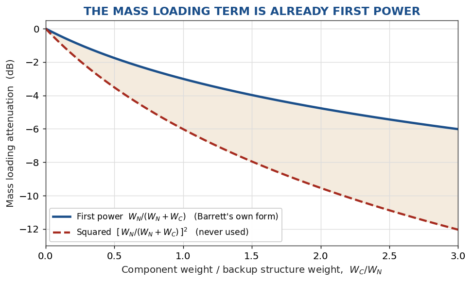
Figure 1. The mass loading bracket in the Barrett equation is a first-power term. A squared version of the same physics has never been used.
How Much Does the Exponent Matter?
Quite a lot, and the penalty grows without bound. In decibels, the difference between the two exponents is numerically equal to the first-power attenuation itself.
| Mass per unit area increase MN / MR | Attenuation, n = 1 | Attenuation, n = 2 | Difference |
|---|---|---|---|
| 1.5 | −1.8 dB | −3.5 dB | 1.8 dB |
| 2 | −3.0 dB | −6.0 dB | 3.0 dB |
| 3 | −4.8 dB | −9.5 dB | 4.8 dB |
| 5 | −7.0 dB | −14.0 dB | 7.0 dB |
| 10 | −10.0 dB | −20.0 dB | 10.0 dB |
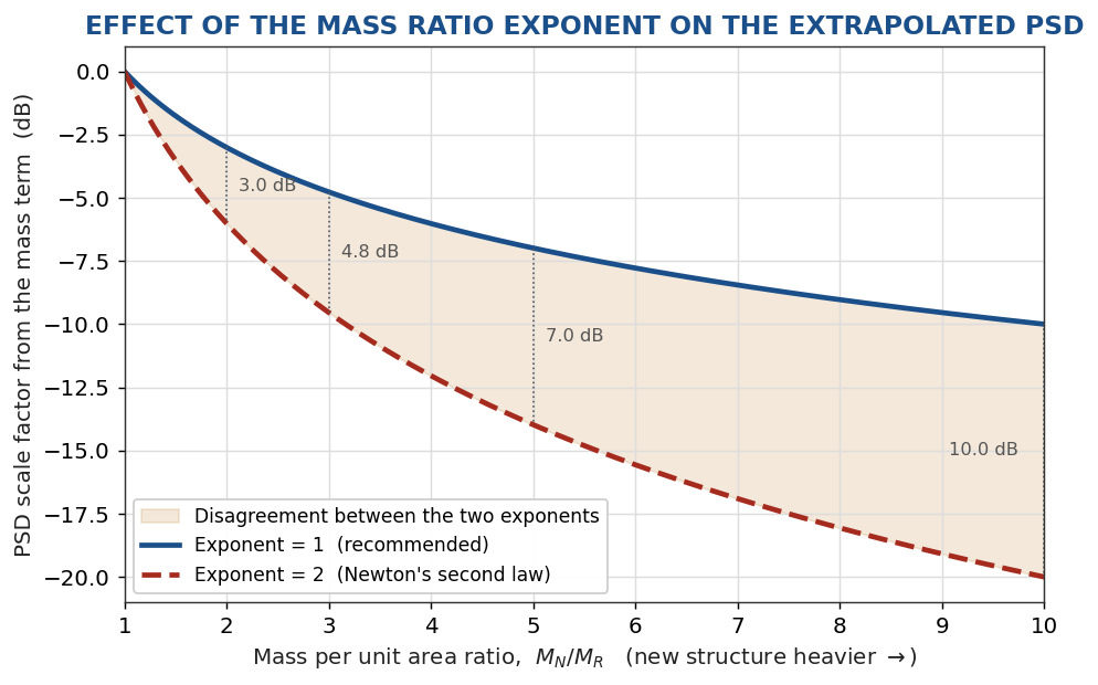
Figure 2. The two exponents agree only at a mass ratio of unity. The shaded band is the disagreement, which reaches 10 dB at a 10:1 ratio.
The practical consequence is that the exponent choice matters least where you need the method least. For a modest extrapolation the two forms differ by a couple of dB, comfortably inside the scatter of the underlying data. For a large extrapolation the squared law can under-predict by 10 dB or more, which is a factor of ten in PSD, a factor of roughly three in GRMS, and a very large factor in fatigue damage. Under-prediction is the dangerous direction.
Worked Example
Take a reference vehicle skin panel environment from the databank with a 0.10 G²/Hz plateau from 100 to 800 Hz, 11.3 GRMS overall. The new vehicle acoustic prediction is 3 dB higher, so the pressure ratio squared is 2.0. The new skin section is three times heavier per unit area, so $M_R/M_N = 1/3$. A 25 lb component is mounted on a 50 lb backup area, so the mass loading factor is 0.667.
| Case | Plateau PSD | Overall |
|---|---|---|
| Reference vehicle | 0.100 G²/Hz | 11.3 GRMS |
| n = 1, no mass loading | 0.067 G²/Hz | 9.2 GRMS |
| n = 1, with mass loading | 0.044 G²/Hz | 7.5 GRMS |
| n = 2, no mass loading | 0.022 G²/Hz | 5.3 GRMS |
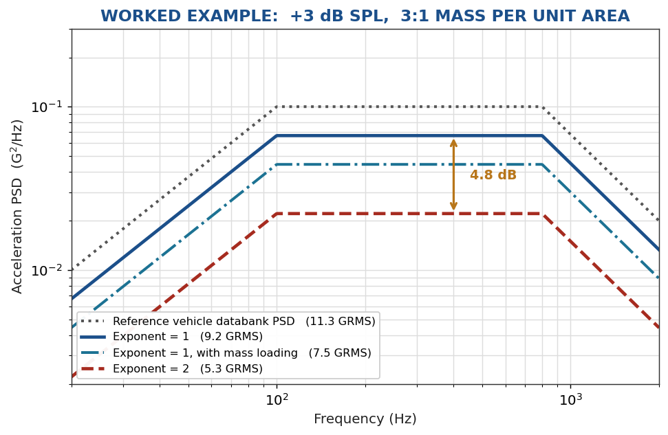
Figure 3. The same reference environment extrapolated two ways. The squared exponent gives a specification 4.8 dB lower across the whole band.
Note that the squared exponent alone accounts for a larger reduction than the mass loading term, and it does so on the strength of an idealization that does not describe the physics of an acoustically driven panel. Writing 5.3 GRMS into a component specification when the defensible answer is 7.5 GRMS is exactly the kind of quiet under-test that shows up later as a screw-back-out or a solder-joint crack during a qualification run.
Practical Cautions
- Check the sense of the mass ratio. It is reference over new, $M_R/M_N$. A heavier new structure must give a lower level. The equation as printed in some sources contains typographical errors in this bracket, and an inverted ratio is easy to overlook because the result still looks like a plausible PSD.
- Match the structural configuration first. Selecting a databank case with the right configuration — skin-stringer to skin-stringer, ring-frame to ring-frame, honeycomb to honeycomb — matters more than the exponent. The exponent is a correction within a family, not a bridge between families.
- Keep the extrapolation modest. The uncertainty in any empirical exponent grows with the distance you push it. A mass ratio beyond about 3:1 is a signal to look for a better reference case, or to switch to SEA, FEM/BEM, or a hybrid method.
- Respect the frequency limits. The Saturn V and Titan III databank spectra span 20 to 2000 Hz. The method has nothing to say below the first panel mode or above the upper limit of the data.
- This is a spatial average. The result is a band-averaged, area-averaged estimate. Envelope it, then apply the normal tolerance limit statistics — P95/50 for maximum predicted environment, with the appropriate flight-to-flight variation term — before it becomes a specification.
- Sanity check in velocity. Convert the result to a velocity spectrum and compare it against the stress-velocity limits for the material. Scaling laws can produce numbers that are arithmetically correct and physically absurd, and a velocity check catches those quickly.
Summary
The exponent of 2 in Barrett’s original derivation is not an error. It is the correct answer to a question about a force-controlled, mass-limited, single-mode response. The exponent of 1 is the correct answer to the question actually being asked: what happens to a resonant, multi-modal, acoustically excited panel when its mass per unit area changes, given that its coupling to the acoustic field changes at the same time. The choice is a modeling decision about the nature of the excitation, not an arithmetic detail, and the flight databanks that the method was built on come down firmly on the side of the first power.
References
- R. E. Barrett, Techniques for Predicting Localized Vibratory Environments of Rocket Vehicles, NASA TN D-1836, Marshall Space Flight Center, October 1963.
- R. C. Ferebee, Using the Saturn V and Titan III Vibroacoustic Databanks for Random Vibration Criteria Development, NASA/TM-2009-215902, Marshall Space Flight Center, July 2009. This is an update to NASA TN D-7159 (1973), with corrections and added Titan III data.
- NASA-HDBK-7005, Dynamic Environmental Criteria.
- MSFC-STD-3676, Development of Vibroacoustic and Shock Design and Test Criteria.
- G. P. Frady et al., Test-Anchored Vibration Response Predictions for an Acoustically Energized Curved Orthogrid Panel with Mounted Components, Marshall Space Flight Center.
- R. H. Lyon and R. G. DeJong, Theory and Application of Statistical Energy Analysis, 2nd edition.
- L. Cremer, M. Heckl and E. Ungar, Structure-Borne Sound.
- Vibrationdata, Vibroacoustics / Statistical Energy Analysis.
Related free ebooks, including the statistical energy analysis and stress-velocity volumes, are collected at Tom’s Ebooks.