Image courtesy of: https://www.rhfs.com

Introduction

Water hammer is one of those phenomena that every piping engineer encounters eventually—and usually remembers. It is the sudden, jarring metallic bang that makes everyone in the control room sit up straight, the distinct shudder transmitted through a facility’s pipe racks, or, in catastrophic cases, the violent rupture of a high-pressure line. Despite the domestic-sounding name, water hammer applies broadly to any liquid flowing in a pressurized system, from liquid natural gas lines to chemical processing plant loops.

Water hammer sits at a fascinating intersection of fluid mechanics, classical acoustics, structural dynamics, and transient shock analysis. The pressure surge originates as an acoustic wave in the fluid, propagates through the complex geometry of the piping network, reflects from boundaries, and ultimately manifests as a severe dynamic load on the piping structure itself.

To safely design or analyze a system, engineers must look beyond simply calculating a peak theoretical pressure. We must understand how that pressure translates into structural force over time.

Historical Background: The Moscow Water Works

The classical mathematical framework for water hammer is attributed to the brilliant Russian scientist and engineer Nikolay Zhukovsky (frequently transliterated as Joukowsky). In the late 1890s, Moscow was upgrading its municipal water supply system, and the cast-iron pipes were suffering mysterious, catastrophic failures.

By conducting large-scale experiments on miles of real pipelines, Zhukovsky developed the foundational law of hydraulic transients:

$$\Delta P = \rho c \Delta V$$

Where:

• $\Delta P$ is the transient pressure change
• $\rho$ is the mass density of the fluid
• $c$ is the acoustic wave speed within the pipe system
• $\Delta V$ is the instantaneous change in fluid velocity

More than a century later, while our computing power has scaled exponentially, every major commercial transient hydraulic code still relies on this elegant relationship as its fundamental starting point.

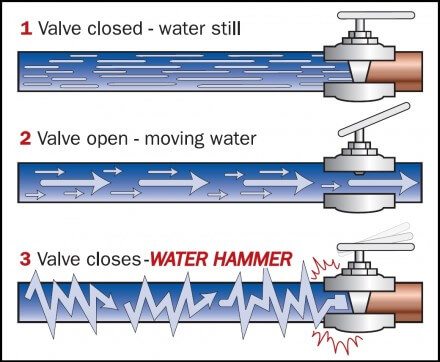
What Is Water Hammer?

At its core, water hammer is a transient hydraulic phenomenon triggered whenever a moving liquid is forced to change velocity rapidly.

Common Triggers in Industrial Systems

• Rapid Valve Operations: Closing an isolation valve too quickly, or the rapid trip of an emergency shutdown valve (ESD).
• Pump Dynamics: A sudden pump trip due to power failure, or abrupt pump startups against an empty or static line.
• Check-Valve Slam: Flow reversal that slams a swing check valve shut just as the reverse velocity peaks.
• System Interactions: Relief valve actuation or a sudden heat exchanger tube rupture.
• Vapor Column Separation: A column of liquid parts due to localized low pressure, creating a vapor pocket. When the flow reverses or the pressure recovers, the vapor pocket collapses violently, causing a massive local pressure spike.

Because liquids are highly incompressible, they possess immense momentum when moving through an industrial system. When that flow is choked off, the fluid’s inertia resists the change. Because no fluid or pipe wall is infinitely rigid, the kinetic energy of the moving fluid is converted into elastic strain energy, generating a high-pressure acoustic wave that races through the piping system.

Water Hammer as an Acoustic Wave

It is helpful to stop thinking of water hammer as a purely hydraulic problem and start thinking of it as an acoustic wave propagation problem. The pressure disturbance is physically analogous to a stress wave propagating through a solid steel bar when struck by a hammer.

In one-dimensional acoustics, the relationship between acoustic pressure and particle velocity is governed by the system’s characteristic impedance:

$$p = Z V$$

For a fluid, the acoustic impedance ($Z$) is defined by its density and wave speed:

$$Z = \rho c$$

Substituting this back yields the Joukowsky equation:

$$\Delta P = \rho c \Delta V$$

Engineers with a background in structural shock and vibration will immediately recognize this as identical to the classical stress-velocity relationship for structural elastic solids:

$$\sigma = \rho c V$$

The physical reality is identical: wave impedance governs the immediate relationship between force (stress/pressure) and velocity. This fundamental connection explains why evaluating fluid velocity changes and time-dependent impulses yields far deeper design insights than tracking macro-accelerations alone.

The Scale of the Joukowsky Prediction

To appreciate why water hammer is so destructive, let us look at the raw numbers for a typical water-carrying pipeline.

• Fluid Density ($\rho$): $\approx 1000\text{ kg/m}^3$
• Acoustic Wave Speed ($c$): $\approx 1000\text{ m/s}$ (accounting for typical pipe wall elasticity)

If a valve is slammed shut, reducing the fluid velocity by a modest $\Delta V = 2\text{ m/s}$, the instantaneous pressure rise is:

$$\Delta P = (1000\text{ kg/m}^3) \times (1000\text{ m/s}) \times (2\text{ m/s}) = 2,000,000\text{ Pa} = 2\text{ MPa}$$

This translates to roughly 300 to 435 psi above normal operating pressure. If your system is already operating near its piping schedule limit, this instantaneous surcharge can easily push fittings past their ultimate tensile strength or cause local structural buckling.

Acoustic Wave Speed in a Fluid-Filled Pipe

The speed at which this pressure wave travels ($c$) is not just a property of the fluid; it is a coupled property of both the fluid and the conduit. A perfectly rigid pipe forces the fluid to bear the full brunt of compression, maximizing wave speed. A flexible pipe wall expands radially, absorbing a portion of the wave energy and slowing it down.

We calculate this coupled wave speed using a modified form of the Korteweg equation:

$$c = \frac{c_{\text{fluid}}}{\sqrt{1 + \frac{D \cdot E_{\text{fluid}}}{e \cdot E_{\text{pipe}}}}}$$

Where:

• $c_{\text{fluid}}$ is the acoustic speed in an infinite body of the fluid ($\approx 1480\text{ m/s}$ for water)
• $D$ is the internal pipe diameter
• $e$ is the pipe wall thickness
• $E_{\text{fluid}}$ is the bulk modulus of the fluid ($\approx 2.2\text{ GPa}$ for water)
• $E_{\text{pipe}}$ is the Young’s modulus of the pipe material ($\approx 200\text{ GPa}$ for steel)

Key Takeaway: Stiffer piping materials (like steel or duplex) yield higher wave speeds, which directly results in higher peak Joukowsky pressure surges. Conversely, flexible materials like HDPE dramatically dampen the wave speed and lower the peak pressure, though they have lower overall pressure ratings.

Characteristic Hydraulic Period

To determine whether a valve stroke is “fast” or “slow,” we must compare the closure time ($t_c$) against the characteristic hydraulic period ($T_h$) of the pipeline:

$$T_h = \frac{2L}{c}$$

Where $L$ is the length of the pipe segment from the valve to the nearest major acoustic reflection point (like a large reservoir, header, or tank). $T_h$ represents the exact round-trip time required for the initial pressure wave to travel to the reflection point, transform into a relief wave, and race back to the valve.

• Fast (Instantaneous) Closure ($t_c < T_h$): The valve fully closes before the reflected relief wave returns. The fluid at the valve experiences the absolute maximum potential Joukowsky pressure rise.
• Slow Closure ($t_c > T_h$): The returning relief wave arrives while the valve is still closing, actively mitigating the pressure buildup. The peak transient pressure will be less than the theoretical Joukowsky maximum.

Wave Reflections and Pressure Amplification

The Joukowsky equation describes a single, isolated traveling wave. Real-world piping networks are complex labyrinths of boundaries. Whenever an acoustic wave hits an obstruction or change in geometry, it reflects and refracts based on the change in acoustic impedance.

Boundary Type	Wave Behavior	Physical Effect
Dead End / Closed Valve	Reflects with the same sign	Doubles the transient pressure magnitude.
Open Reservoir / Large Header	Reflects with the opposite sign	Inverts a pressure peak into a pressure drop (relief wave).
Diameter Reduction	Partial reflection	Transmits a higher pressure wave forward into the smaller pipe.
Tees and Branches	Wave division	Splits the acoustic energy across multiple paths, reducing local magnitude.

Because these waves bounce back and forth, they can constructively interfere. If multiple pressure peaks stack on top of one another, the local pressure can drastically exceed the original Joukowsky prediction. This is why engineering standards require modeling complex systems with transient software (e.g., AFT Impulse) rather than relying solely on hand calculations.

Structural Loading at Pipe Bends

Once we know the transient pressure profile over time, we must translate that fluid pressure into a physical structural force.

Uniform static pressure inside a straight pipe is self-equilibrating—it exerts equal radial force everywhere. However, when an acoustic wave travels through a pipe bend or elbow pair, it creates a transient force imbalance.

As the sharp pressure front enters an elbow, it applies a force to the turning plane of that elbow. Until that wave travels down the span length ($L_{\text{span}}$) to reach the next elbow, the system is structurally unbalanced.

The peak net dynamic force acting on that piping segment is:

$$F = \Delta P \cdot A$$

Where $A$ is the internal cross-sectional area of the pipe. This unbalance exists only during the brief window it takes for the wave front to traverse the distance between the two bends. Therefore, the force pulse duration ($\tau$) is calculated as:

$$\tau = \frac{L_{\text{span}}}{c}$$

The moment the wave reaches the second elbow, the pressures balance out, and the net structural driving force drops back to near zero. This rapid “loading-then-unloading” profile creates a distinct shock pulse.

Hydraulic Amplification vs. Structural Amplification

Engineers often conflate fluid amplification with structural amplification. They are entirely separate phenomena governed by different physical parameters.

1. Hydraulic Amplification

• Driven by: Fluid acoustics, wave stacking, and impedance mismatches.
• Governing Parameter: System geometry and boundary reflection coefficients.
• Result: An increase in the raw fluid pressure ($\Delta P$).

2. Structural Amplification

• Driven by: Structural resonance and structural dynamics.
• Governing Parameter: The ratio of the pulse duration to the structural natural period ($\tau/T$).
• Result: Structural displacement, high bending moments, and stress failures in supports.

A system can experience massive hydraulic pressures but minimal structural deflection if the pulse is over too quickly. Conversely, a modest hydraulic pressure pulse can tear a pipe rack apart if its duration perfectly matches the structural resonance of the piping system.

Dynamic Amplification and Pulse Regimes

To evaluate how a piping system responds to a water hammer force pulse, we idealize the pipe span as a single-degree-of-freedom (SDOF) structural system subjected to a rectangular force pulse of magnitude $F_0$ and duration $\tau$.

The structural response is characterized by the Dynamic Load Factor (DLF), defined as the ratio of maximum dynamic displacement to equivalent static displacement ($x_{\text{max}} / x_{\text{static}}$). The response falls into three distinct regimes based on the ratio of pulse duration to the structural natural period ($\tau/T$):

The Three Structural Response Regimes

1. Quasi-Static Regime ($\tau/T \gg 1$): The force pulse lasts a long time relative to the structure’s ability to flex. The structure has ample time to deform, the response tracks the force profile exactly, and $\text{DLF} \approx 1.0$.
2. Dynamic / Resonant Regime ($\tau/T \approx 0.5$): The force unloads at the exact worst moment—just as the structure is flexing forward. The structural response amplifies dramatically, reaching a peak theoretical $\text{DLF} \approx 2.0$.
3. Impulsive Regime ($\tau/T \ll 1$): The force pulse is over in a flash. The structure barely has time to register the force before it disappears. In this regime, the peak displacement depends entirely on the total impulse (the area under the force-time curve, $F_0 \tau$) rather than the peak force magnitude alone.

Reader Question: Heat Exchanger Tube Rupture and the $\tau/T < 0.01$ Criterion

The Scenario

“Is there published or theoretical support for screening out water-hammer-induced structural loads on attached piping whenever the pulse-duration ratio falls below $\tau/T < 0.01$? The scenario involves a high-pressure heat exchanger tube rupture venting into a low-pressure shell, generating rapid structural pulses in the surrounding piping.”

This is an exceptional question that requires evaluating structural dynamics against real plant conditions. The short answer is yes, the underlying physics is absolutely correct and defensible, though you will not find it explicitly named as an arbitrary safety rule in a standard design code.

Let’s break down the mathematical derivation and physical justification for this screening criterion.

Analytical Derivation of the $\tau/T = 0.01$ Response

For an undamped, un-preloaded SDOF system subjected to a sudden rectangular force pulse, classical structural dynamics dictates that during the loading phase ($t \le \tau$), the displacement response is:

$$x(t) = \frac{F_0}{k}(1 – \cos \omega t)$$

The absolute maximum response occurs after or at the end of the short pulse duration. For short pulses ($\tau/T \le 0.5$), the maximum dynamic displacement is reached during the free-vibration phase and is defined by:

$$x_{\text{max}} = \frac{F_0}{k} \cdot 2\sin\left(\frac{\pi \tau}{T}\right)$$

Therefore, the Dynamic Load Factor is exactly:

$$\text{DLF} = 2\sin\left(\frac{\pi \tau}{T}\right)$$

When the pulse duration is exceptionally small relative to the structural period ($\tau/T \ll 1$), we can apply the small-angle small-argument approximation ($\sin \theta \approx \theta$):

$$\sin\left(\frac{\pi \tau}{T}\right) \approx \frac{\pi \tau}{T}$$

Substituting this back into our DLF equation gives us a purely linear relationship for the impulsive regime:

$$\text{DLF} \approx 2\pi \left(\frac{\tau}{T}\right)$$

Now, let us evaluate this linear approximation at the reader’s proposed screening threshold of $\tau/T = 0.01$:

$$\text{DLF} \approx 2\pi(0.01) \approx 0.0628$$

The Structural Reality

At $\tau/T = 0.01$, the maximum dynamic load felt by the pipe rack, anchors, and supports is only 6.3% of the equivalent static load. The structure barely budsges.

Energy Interpretation: Why the Strain Energy Tells the Real Story

We can look at this through an energy lens to add a layer of engineering confidence. The mechanical strain energy ($U$) stored in a deflected piping system scales with the square of its displacement ($U \propto x^2$).

If we compare the dynamic strain energy accumulated during this ultra-short pulse to the strain energy of a static application of the same peak force, we find:

$$\frac{U_{\text{dynamic}}}{U_{\text{static}}} = (\text{DLF})^2 = (0.0628)^2 \approx 0.0039$$

The piping system absorbs less than 0.4% of the energy it would absorb if that force were applied statically. Because structural failure is fundamentally an energy-absorption and strain-limit problem, an event that transmits less than 0.4% energy is an ideal candidate for engineering screening.

Validation in Engineering Literature

While a specific cutoff like $\tau/T < 0.01$ is rarely written into codes as an ironclad exemption, the foundational literature explicitly maps out and validates this behavior:

• Biggs, Introduction to Structural Dynamics (1964): Provides the definitive, classical DLF charts for rectangular, triangular, and triangular-decay pulses. At a time duration ratio of $0.01$, all curves converge asymptotically toward zero response.
• Chopra, Dynamics of Structures: Outlines shock response spectra (SRS). It establishes that for small normalized durations, the system response is entirely impulse-controlled ($I = F_0\tau$), and peak force magnitude loses its physical engineering relevance.
• UFC 3-340-02 (Formerly TM 5-1300) | Structures to Resist the Effects of Accidental Explosions: This military structural blast design manual uses pressure-impulse ($P-I$) diagrams extensively. It formalizes the “impulsive realm” where structural damage is independent of peak pressure, validating the use of brief pulse durations to screen out macro-structural failures.
• Wilcox & Walters, Evaluating Dynamic Loads in Piping Systems Caused by Waterhammer (2012): Directly links the hydraulic wave transit time across elbow pairs ($\tau = L/c$) to dynamic pipe stress modeling, confirming that ultra-short spans experience minimal dynamic coupling.

The Hidden Conservatism: 3D Attenuation in Tube Ruptures

Using a 1D hand calculation for a heat exchanger tube rupture actually introduces massive structural conservatism.

A standard water hammer event starts as a flat, planar wave across the entire cross-section of a pipe. A tube rupture, however, begins as a highly localized, point-source fluid jet deep inside a dense matrix of surrounding tubes, baffles, and shell space.

Before that pressure wave can exit the exchanger nozzles and load your external piping, it undergoes severe physical attenuation:

1. Geometric Spreading: The wave expands spherically outward from the burst tube, dropping in energy density instantly.
2. Baffle and Tube Bundle Scattering: The wave front strikes hundreds of internal shell-side tubes and baffles, shattering the coherent wave front and scattering the energy.
3. Turbulent Dissipation and Volume Dampening: The local fluid volume acts as an energy buffer, absorbing the initial acoustic shock before it can cleanly couple into the connected process lines.

Therefore, modeling the event as a pristine, un-attenuated 1D Joukowsky wave hitting an external elbow pair provides a major safety factor over real-world conditions.

Practical Engineering Screening Workflow

If you are tasked with auditing a piping system for transient water hammer or tube rupture loads, you can use this structured screening workflow to save hundreds of hours of simulation time:

Summary

Water hammer is an acoustic phenomenon disguised as a hydraulic problem. While the fluid pressure rise can be immense, the structural damage it inflicts depends entirely on time-scale matching.

When analyzing short pipe spans or fast transient events like tube ruptures, the force pulse duration ($\tau$) is often tiny compared to the structural natural period ($T$). If $\tau/T < 0.01$, the system is deep within the impulsive regime. Classical structural dynamics proves that the resulting Dynamic Load Factor will be less than $0.063$, meaning the piping system reacts to less than 6% of the force it would experience statically.

While not written out explicitly as an arbitrary code clause, using $\tau/T < 0.01$ as a screening threshold is a rigorous, physics-backed engineering approach that safely filters out benign events, allowing teams to focus their computational resources on deep, resonant structural risks.

– Tom Irvine