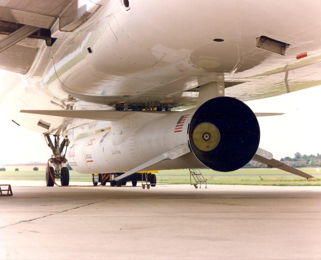
Cut a rectangular hole in an aerodynamic surface and fly it at high subsonic or supersonic speed, and the hole will sing. Not quietly. Overall sound pressure levels inside a fighter weapon bay routinely exceed 160 dB, and the energy is not spread evenly across the spectrum. It is concentrated into a set of sharp tones whose frequencies follow a simple, remarkably durable formula published by J. E. Rossiter at the Royal Aircraft Establishment in 1964.
Structural dynamicists meet these tones in weapon bays, landing gear wells, open hatches and access panels, gaps and steps in launch vehicle skirts, pantograph recesses on high-speed trains, and — at a much smaller scale and lower speed — the throb you feel when you open one rear window in a moving car. The mechanism is the same in every case. What changes is where the tones land relative to the structural modes, and that is what decides whether the cavity is a nuisance or a fatigue problem.
The Feedback Loop
Rossiter’s insight was that cavity tones are not organ-pipe resonances of the cavity volume. They are the product of a closed feedback loop between the flow and its own acoustic radiation.
The boundary layer separates at the forward lip and spans the opening as a free shear layer. That shear layer is unstable, and it rolls up into discrete vortices which convect downstream at some fraction of the freestream velocity. When a vortex reaches the aft bulkhead it impinges, and the impingement radiates an acoustic pulse. That pulse propagates upstream — inside the cavity, through relatively still air — and arrives back at the forward lip, where the shear layer is most receptive to disturbance. The arriving pulse triggers the formation of the next vortex, and the loop closes.
Tones occur at the frequencies for which the total loop phase — convection downstream plus acoustic propagation upstream — is an integer number of cycles. That integer is the mode number $m$, and the modes are conventionally labelled $m = 1, 2, 3, \dots$
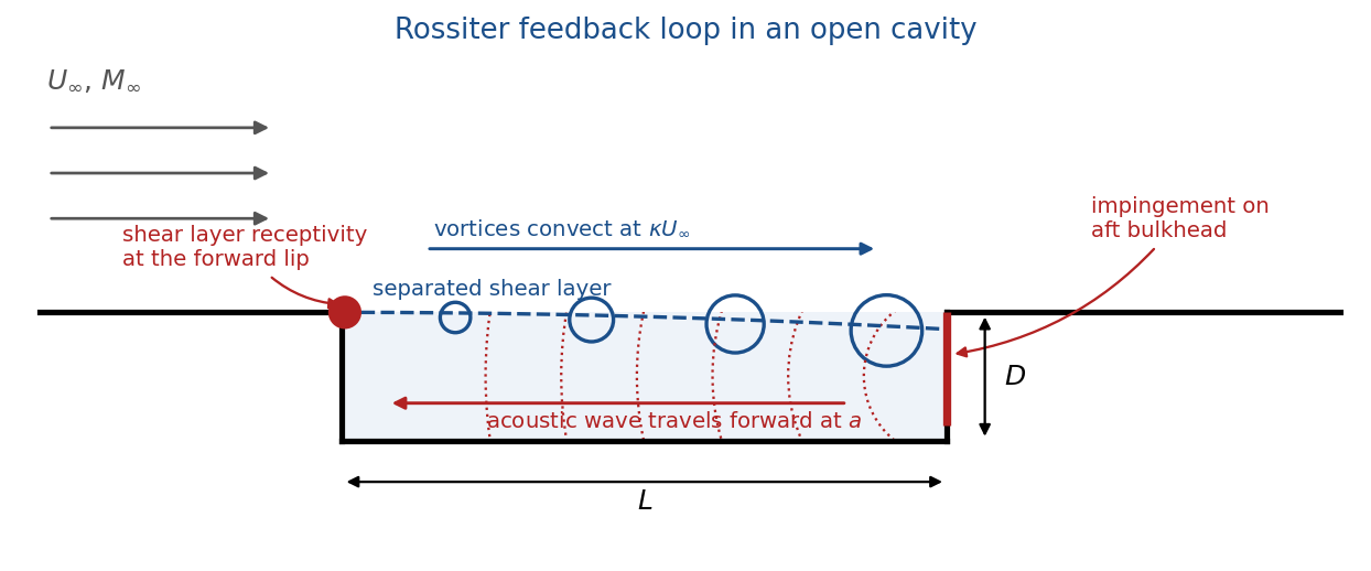
Figure 1. The Rossiter feedback loop. Vortices convect aft at $\kappa U_\infty$; the acoustic disturbance from aft-wall impingement returns forward at the speed of sound.
The Rossiter Formula
Writing the loop-phase condition out and non-dimensionalizing on cavity length $L$ and freestream velocity $U_\infty$ gives the Strouhal number of the $m$-th tone:
$$ St_m \; = \; \frac{f_m L}{U_\infty} \; = \; \frac{m – \alpha}{ M_\infty + \dfrac{1}{\kappa} } $$
There are only two empirical constants. The parameter $\kappa$ is the ratio of vortex convection velocity to freestream velocity, and $\alpha$ is a phase lag accounting for the delay between the acoustic wave arriving at the lip and the resulting vortex being shed. Rossiter fitted $\kappa \approx 0.57$ and $\alpha \approx 0.25$ to wind tunnel data, and those values have held up well enough that they are still the default sixty years later.
Note what is absent. Cavity depth does not appear. Neither does Reynolds number, boundary layer thickness, or anything about the cavity contents. It is a length scale, a velocity, and two numbers. That parsimony is the reason the formula is still in daily use.
The Heller-Bliss Correction
The original derivation assumes the upstream-travelling acoustic wave moves at the freestream speed of sound. It does not. The air inside the cavity is nearly stagnant, so its static temperature has recovered toward the stagnation temperature, and the local speed of sound is correspondingly higher. Heller, Holmes and Covert corrected for this in 1971 by replacing $M_\infty$ in the denominator with the Mach number referenced to the recovered internal sound speed:
$$ St_m \; = \; \frac{f_m L}{U_\infty} \; = \; \frac{m – \alpha}{ \dfrac{M_\infty}{\sqrt{\,1 + \frac{\gamma – 1}{2} M_\infty^{2}\,}} \; + \; \dfrac{1}{\kappa} } $$
Here $\gamma = 1.4$ is the ratio of specific heats. The correction is negligible at low subsonic speeds and becomes significant as Mach number climbs:
| $M_\infty$ | $St_2$, Rossiter | $St_2$, Heller-Bliss | Difference |
|---|---|---|---|
| 0.70 | 0.713 | 0.722 | 1.3 % |
| 0.90 | 0.659 | 0.676 | 2.5 % |
| 1.20 | 0.592 | 0.622 | 5.1 % |
| 1.60 | 0.522 | 0.573 | 9.8 % |
Table 1. Effect of the compressibility correction on the second mode, $\kappa = 0.57$, $\alpha = 0.25$.
A ten percent frequency error does not sound like much until you remember what these tones are being compared against. If a Rossiter tone is being checked for coincidence with a lightly damped structural mode, ten percent is the difference between a hit and a miss.
Open, Transitional, and Closed Cavities
The formula applies to open cavity flow, in which the shear layer bridges the opening and reattaches on the aft bulkhead. That regime holds for roughly $L/D < 10$. For $L/D$ beyond about 13 the shear layer dives into the cavity, reattaches on the floor, and separates again ahead of the aft wall — a closed cavity. Closed cavities do not sustain the feedback loop and are acoustically much quieter, but they impose a severe streamwise static pressure gradient that drives large nose-up pitching moments on a released store. Between the two lies a transitional regime that switches back and forth with small changes in Mach number, which is the worst of both worlds and is generally designed out.
Worked Example: A Fighter Weapon Bay
Take a bay sized to carry a 2000 lb class weapon, $L = 4.27$ m (14 ft), at 30,000 ft on a standard day where the freestream speed of sound is 303 m/s. Applying the Heller-Bliss form:
| $M_\infty$ | $U_\infty$ (m/s) | $m = 1$ | $m = 2$ | $m = 3$ | $m = 4$ |
|---|---|---|---|---|---|
| 0.70 | 212 | 15.4 Hz | 35.9 Hz | 56.4 Hz | 76.9 Hz |
| 0.85 | 258 | 17.7 Hz | 41.4 Hz | 65.1 Hz | 88.7 Hz |
| 0.95 | 288 | 19.2 Hz | 44.9 Hz | 70.5 Hz | 96.2 Hz |
| 1.20 | 364 | 22.7 Hz | 53.0 Hz | 83.3 Hz | 113.6 Hz |
| 1.60 | 485 | 27.9 Hz | 65.0 Hz | 102.2 Hz | 139.3 Hz |
Table 2. Heller-Bliss tone frequencies, $L$ = 4.27 m, 30,000 ft standard day.
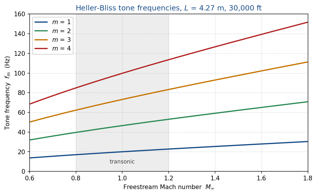
Figure 2. Tone frequencies sweep upward with Mach number. A single structural mode can be crossed by several Rossiter modes over the course of one acceleration.
Figure 2 contains the operational point that matters most. The tone frequencies are not fixed. They sweep upward roughly in proportion to velocity, so during a transonic acceleration the whole comb of tones marches through the structural band. Any given structural mode will be swept through by mode 1, then mode 2, then mode 3, in succession. The dwell time at each coincidence is set by the acceleration rate, and the response is a swept-sine problem, not a stationary random problem.
Tones on a Broadband Floor
A measured cavity spectrum is not a line spectrum. It is a set of finite-width peaks riding on a substantial broadband floor generated by the turbulent shear layer itself. Individual tones commonly stand 10 to 25 dB above the floor, with the second and third modes usually dominant. Depth modes — transverse standing waves at $f_n = (2n-1)\,a/(4D)$ for a quarter-wave cavity — can also appear, and can couple with the Rossiter modes when they are close.
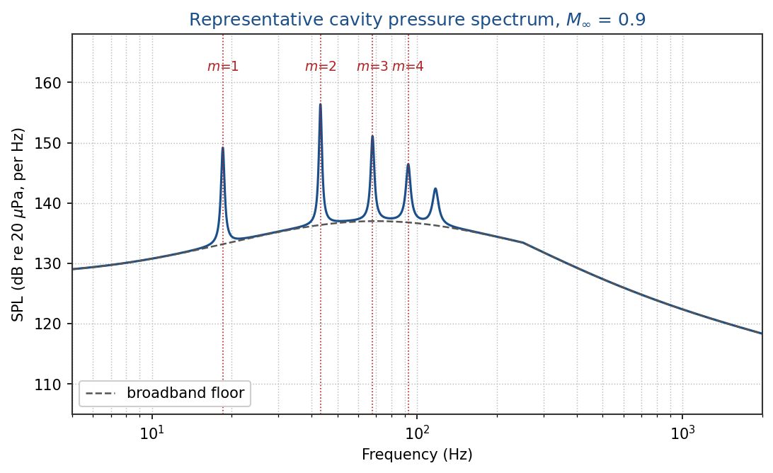
Figure 3. Representative cavity spectrum, $M_\infty$ = 0.9, showing four Rossiter tones on the shear-layer broadband floor.
Amplitude scales with dynamic pressure. The fluctuating pressure coefficient $p_{rms}/q$ is roughly constant for a given geometry and Mach number, typically in the range 0.05 to 0.20. At $q$ = 1000 psf with a coefficient of 0.10, $p_{rms}$ = 0.69 psi, which is 168 dB. Drop to $q$ = 400 psf and the same coefficient gives 160 dB. Since the pressure PSD goes as $q^2$, and fatigue damage goes as stress to the power $b$, damage per unit time in a cavity scales as $q^{\,b}$. Between those two conditions, with $b = 4$, that is a factor of 39 in damage rate per second of exposure. Cavity duty cycles have to be binned by dynamic pressure. Lumping them is not conservative — it is simply wrong in an unknown direction.
One further caution on amplitude. Cavity pressure is measurably non-Gaussian, with kurtosis above 3. Damage estimates that assume a Gaussian process and a Rayleigh peak distribution will under-predict, and the tonal content makes the Rayleigh assumption doubly suspect: a lightly damped mode driven at a discrete tone produces peaks that are closer to sinusoidal than Rayleigh, with a tighter distribution and far more cycles near the maximum.
Why This Is a Structural Dynamics Problem
The phrase “160 dB acoustic environment” invites the wrong toolkit. Statistical energy analysis, diffuse field assumptions, third-octave band levels — all of that belongs to problems with high modal density. A large cavity does not have high modal density where its energy is, because Rossiter frequencies scale as $1/L$, and a large cavity puts its tones low.
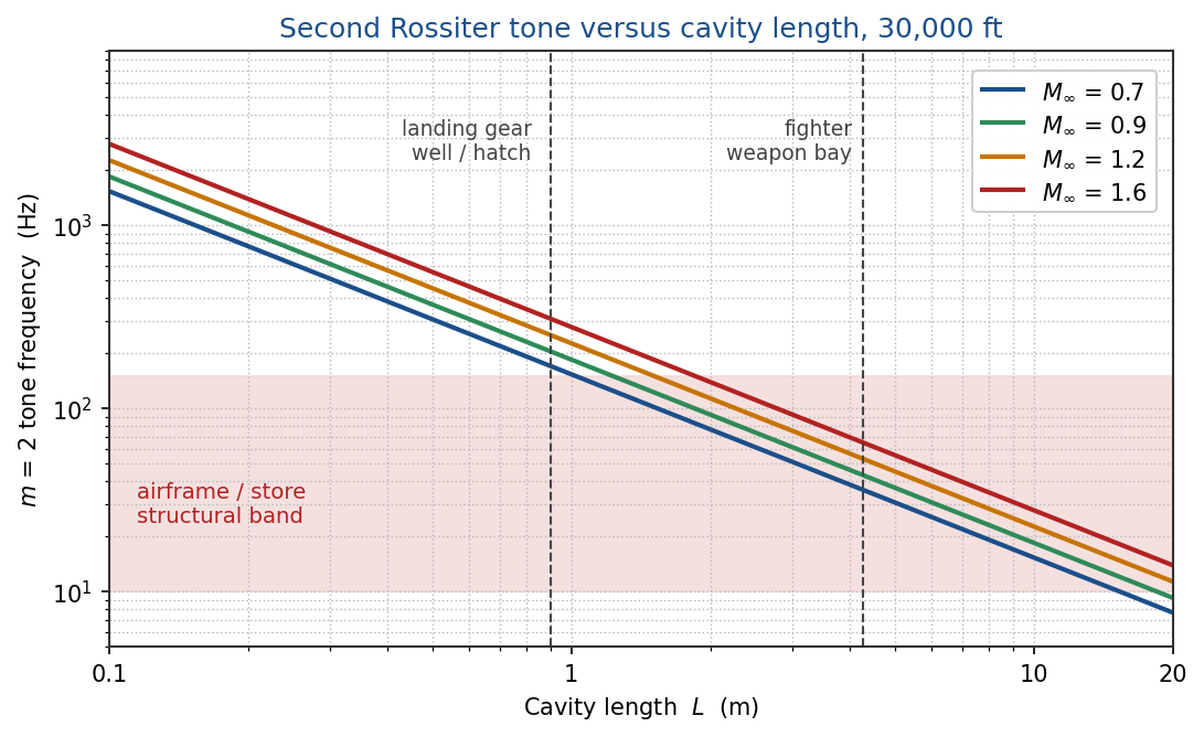
Figure 4. The $m$ = 2 tone versus cavity length. Small cavities put their tones safely above the structural band. Large ones put them squarely inside it.
Figure 4 makes the scaling argument directly. A hatch or gear well under a metre long generates tones in the hundreds of hertz, well above most primary structural modes, and can reasonably be treated as an acoustic fatigue problem for skin panels. A four-metre weapon bay generates tones between 20 and 140 Hz — right on top of rigid-body store modes on their suspension, first and second free-free bending of a carried store, and door panel modes. That is a modal, deterministic, coupled problem. It wants a finite element model with a boundary element or wavenumber-domain pressure loading, not a diffuse-field energy balance.
Duration and Damage
Cavity exposure is usually brief. Doors open, something is released, doors close — a matter of seconds. It is tempting to dismiss such short exposures against hundreds of hours of ordinary flight. That instinct is wrong, and the arithmetic shows why. Damage rate scales as $(G_{rms})^{\,b}$, so a level increase of $\Delta$ dB in PSD corresponds to an amplitude ratio $r = 10^{\Delta/20}$ and a damage rate ratio of $r^{\,b}$. One second of cavity exposure is then equivalent to the following amount of benign-condition exposure:
| $\Delta$ PSD | Amplitude ratio $r$ | $b$ = 4 | $b$ = 6 |
|---|---|---|---|
| 15 dB | 5.6 | 0.28 hr | 8.7 hr |
| 20 dB | 10.0 | 2.8 hr | 278 hr |
| 25 dB | 17.8 | 27.8 hr | 8,800 hr |
| 30 dB | 31.6 | 278 hr | 278,000 hr |
Table 3. Benign-condition exposure equivalent to one second of cavity exposure, by level increment and S-N exponent.
At a 25 dB increment with $b$ = 4, thirty-six seconds of cumulative cavity exposure equals a thousand hours of ordinary flight. For any plausible cavity level, a handful of seconds can dominate the fatigue life. Note also that the exposure is cycle-poor: five seconds at 25 Hz is about 125 cycles, which is nowhere near the asymptotic regime where spectral damage methods such as Dirlik are on firm ground. For a segment that short I would run several time-domain realizations and examine the distribution of damage, rather than trusting a single spectral estimate — and I would check peak response against static allowables separately, because 125 high-amplitude cycles is as much a strength question as a fatigue question.
Suppression
Every practical suppression scheme attacks the same link in the loop: the coherence of the shear layer. If the vortices arriving at the aft bulkhead are diffuse and disorganized rather than compact and periodic, the returning acoustic pulse is weak and the loop cannot sustain itself.
Passive devices at the forward lip do this by thickening the shear layer and lifting it clear of the aft wall. Spoilers, sawtooth serrations, fences, and the classic rod-in-crossflow all work on this principle and can deliver 10 to 20 dB of tone reduction, at the cost of drag and, for a stealth platform, of a geometric feature nobody wants. Active methods — steady or pulsed blowing at the lip, or closed-loop control driven by an aft-wall pressure sensor — can do better and can adapt across the envelope, but add complexity and bleed air. Passive treatment remains the default in fielded systems.
Practical Notes
A few points that repeatedly cause trouble in practice. First, use the cavity length that the flow sees, not a drawing dimension: partially open doors, a protruding store, and a stepped aft bulkhead all change the effective $L$. Second, $\kappa$ and $\alpha$ are fitted constants, not physical laws; where measured data exist, refit them rather than accepting 0.57 and 0.25. Third, the tone frequencies move with flight condition, so a Welch-averaged PSD taken over a long record during an acceleration will smear the tones into a broad hump and badly under-state the peak levels — use short-time analysis or a spectrogram, and resist the urge to average. Fourth, a store in the bay is not a passive occupant; it changes the effective cavity geometry, and a bay measured empty is not the same bay when loaded.
References
Rossiter, J. E., Wind-Tunnel Experiments on the Flow over Rectangular Cavities at Subsonic and Transonic Speeds, RAE Technical Report 64037, 1964; also ARC R&M 3438, 1966.
Heller, H. H., Holmes, D. G., and Covert, E. E., “Flow-Induced Pressure Oscillations in Shallow Cavities,” Journal of Sound and Vibration, Vol. 18, 1971.
Heller, H. H., and Bliss, D. B., “The Physical Mechanism of Flow-Induced Pressure Fluctuations in Cavities and Concepts for Their Suppression,” AIAA Paper 75-491, 1975.
Plentovich, E. B., Stallings, R. L., and Tracy, M. B., Experimental Cavity Pressure Measurements at Subsonic and Transonic Speeds, NASA Technical Paper 3358, 1993.
Cattafesta, L. N., Song, Q., Williams, D. R., Rowley, C. W., and Alvi, F. S., “Active Control of Flow-Induced Cavity Oscillations,” Progress in Aerospace Sciences, Vol. 44, 2008.
Related material, including tutorials on acoustic fatigue, statistical energy analysis, and rainflow-based damage methods, is available in the free ebook collection at Tom’s Ebooks.