
A large external store is to be carried under an aircraft wing on a pylon. The airframe manufacturer runs its buffet analysis and hands the store vendor an acceleration power spectral density at the pylon/wing interface. The vendor applies that PSD as base excitation to a finite element model of the pylon and store, usually via the large seismic mass method, recovers stresses, rainflow counts them, and carries the resulting spectrum into a NASGRO crack growth analysis. The chain is familiar, every link in it is standard practice, and the answer can still be wrong by an order of magnitude in fatigue damage. This post works through why, using a two-degree-of-freedom model where the exact answer is available for comparison. It then explains what a Craig-Bampton reduction actually is, quantifies how many modes such a reduction has to carry, and shows that the reduced-model exchange being proposed here is not an import from the spacecraft world at all — it is established aircraft practice that has simply never been pointed at the store vibration environment.
The Interface PSD Is a Response, Not a Boundary Condition
The root problem is that an acceleration PSD at a structural interface has no meaning apart from the impedance that produced it. Enforcing it as motion — through a seismic mass, a Single-Point Constraint Displacement (SPCD), or any other device — asserts that the driving point impedance on the source side is infinite. The seismic mass will supply whatever force is required to hold the specified acceleration, without limit. In the real aircraft, when the store passes through one of its own resonances it draws a large reactive force from the wing, the wing yields to it, and the interface acceleration notches. The enforced motion model has no mechanism to notch. It delivers a force spike instead.
For a single interface degree of freedom the relationship is exact and well known from force limited vibration testing. If $M_S(\omega)$ is the driving point apparent mass of the source, $M_L(\omega)$ is the apparent mass of the load, and $S_{AA}^{free}$ is the acceleration PSD the source would exhibit at that point with no store attached, then the coupled interface acceleration is
$$S_{AA}^{coupled}(\omega) \; = \; \frac{S_{AA}^{free}(\omega)}{\left| \, 1 + \dfrac{M_L(\omega)}{M_S(\omega)} \, \right|^{2}}$$The notch depth is set entirely by the apparent mass ratio. At the store’s fixed-base resonance the load apparent mass rises by roughly its dynamic amplification factor, the ratio becomes large, and the interface acceleration collapses. That collapse is not a modeling nicety. It is the single most important feature of the environment, and it is precisely what an unnotched specification omits.
A Two-Degree-of-Freedom Demonstration
Consider a source subsystem representing the wing effective modal mass at the station, carrying a load subsystem representing the pylon and store. Buffet is applied as a force on the source. The parameters are deliberately ordinary for a heavy store installation.
| Parameter | Value | Comment |
|---|---|---|
| Wing effective modal mass | 1000 lbm | at the pylon station, single mode |
| Pylon plus store mass | 2000 lbm | mass ratio 2.0 |
| Wing mode, no store | 12 Hz | 3% critical damping |
| Store on pylon, fixed base | 35 Hz | 3% critical damping |
| Buffet force PSD | flat, 5 to 100 Hz | fourth-power rolloff outside the band |
Coupling this pair moves the system modes to 6.84 Hz and 61.42 Hz. Neither uncoupled frequency survives. An analyst who was handed an interface spectrum generated without the store, and who then hunts for the wing mode at 12 Hz in his own results, is looking for something that does not exist in the flight article.
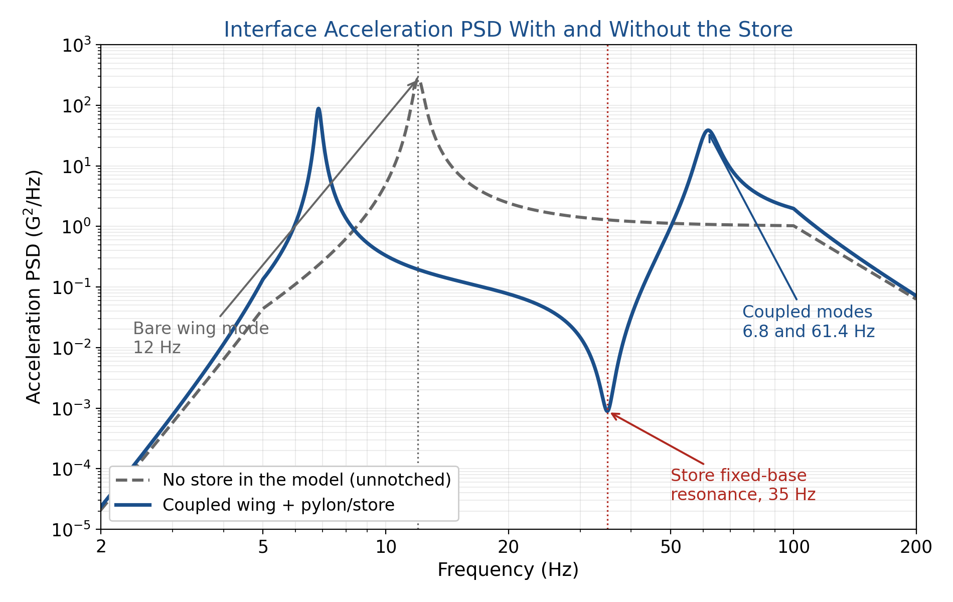
Figure 1 shows the two interface spectra. The broadband RMS levels differ by only 0.66 dB — 20.97 G against 22.62 G — which is why this error survives review so often. The overall number looks fine. But at 35 Hz, where the store’s own resonance lives, the apparent mass ratio reaches 37.8 and the unnotched spectrum sits 31.6 dB above the truth. All of the disagreement is concentrated at exactly the frequency that governs the store’s internal loads.
What the Enforced Motion Model Predicts
Figure 2 gives the store center of gravity response four ways: the exact coupled solution, base drive using the unnotched no-store spectrum, base drive using an envelope of the two spectra, and base drive with semi-empirical force limiting applied at $C^2 = 2$.
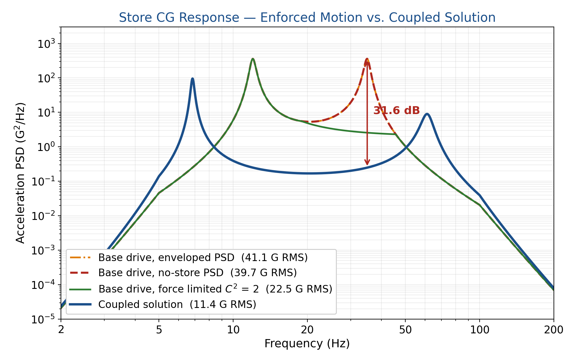
Damage is estimated with the narrowband proxy $D \propto n_0 \sigma^{m}$ at $m = 3$, using the zero crossing rate $n_0 = \sqrt{m_2/m_0}$ of each response spectrum. This understates the spread that a full rainflow analysis would show, since it does not credit the change in peak distribution, but it is sufficient to make the point.
| Case | RMS (G) | $n_0$ (Hz) | dB vs. truth | Damage ratio |
|---|---|---|---|---|
| Coupled solution | 11.37 | 51.8 | 0.00 | 1.00 |
| Base drive, no-store PSD | 39.74 | 30.7 | +10.87 | 25.3 |
| Base drive, enveloped PSD | 41.06 | 32.5 | +11.15 | 29.6 |
| Base drive, force limited $C^2 = 2$ | 22.51 | — | +5.93 | 2.96 |
| Base drive, exact coupled PSD | 11.37 | 51.8 | 0.00 | 1.00 |
The unnotched base drive over-predicts store response by 10.9 dB on RMS and by a factor of 25 on damage. Enveloping makes it slightly worse, which is worth dwelling on: enveloping is normally a conservative and defensible act, but here it fills in the physical notch, and the notch was the real environment.
An Important Qualification
The last row of the table deserves emphasis, because it cuts against the reflexive criticism of base drive. If the interface spectrum is derived from the coupled system with this store installed, and the interface is a single point in a single axis, then base driving with that spectrum reproduces the coupled store response exactly — 0.00 dB, not approximately. This is not a coincidence. The load subsystem’s equation of motion under enforced base motion is identical to its equation within the coupled system, so if the base motion is correct the response is correct. The seismic mass method is not inherently wrong.
What is wrong is the practical situation the method is normally used in. The exactness evaporates as soon as any of the following is true, and at least one of them is always true:
- The spectrum was generated without the store, with a different store, or with a different fuel or expenditure state.
- The spectrum is an envelope across stations, configurations, or flight conditions.
- The attachment is multi-point — lugs, hooks, and preloaded sway braces — rather than a single driven node. Driving several points identically, or through an RBE2 spider, enforces a rigid interface that the real installation does not have, and discards the relative motion and phase among the attachments.
- The specification is single-axis while the real interface motion is six degrees of freedom with correlation among them.
- The vendor’s assumed damping differs from the damping used by the airframer to generate the spectrum, which shifts the notch depth.
So the honest statement is narrower and more useful than “base drive over-predicts.” It is this: base drive is exact when the enforced motion is the true coupled motion at every interface degree of freedom, and the error is governed by how far the specified motion departs from that. Enveloping, generic spectra, and rigid interfaces are the mechanisms of departure.
The Interface Force
Figure 3 plots the quantity the seismic mass never constrains. The coupled interface force is 22,748 lbf RMS. Under unnotched enforced motion it is 79,489 lbf RMS, and at the store resonance the force PSD is more than three orders of magnitude high. Nothing in the analysis flags this, because force is not what was specified.
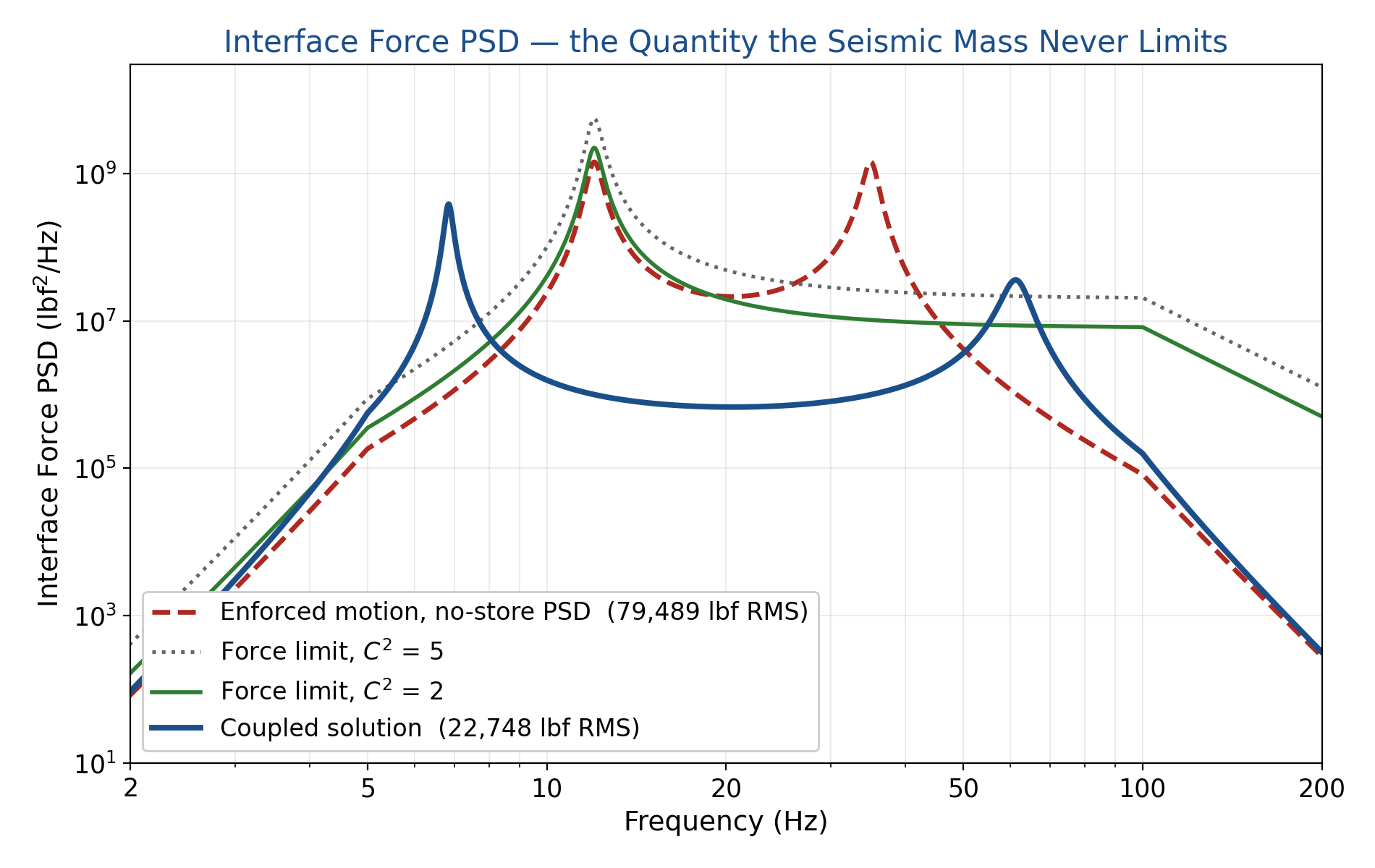
This is the same pathology that force limited vibration testing was invented to cure on the shaker, and the cure transfers directly to the analysis. The semi-empirical limit is
$$S_{FF}(f) \; = \; C^{2} \, M_{o}^{2} \, S_{AA}(f)$$where $M_o$ is the total mass of the load and $C^2$ is normally taken between 2 and 5. Applying $C^2 = 2$ to the unnotched spectrum in this example pulls the over-prediction from 10.9 dB down to 5.9 dB and the damage ratio from 25 to 3. That is a large improvement for very little work, and it should be regarded as the minimum defensible treatment rather than as a refinement. It is also not a substitute for the coupled analysis: the value of $C^2$ that would reproduce the true interface force here is about 0.2, well below the conventional range, because the mass ratio is large. The semi-empirical constant is a bound, not a prediction.
Two Further Problems, Specific to Fracture Analysis
Stationarity and the peak distribution. Buffet is intermittent. It occurs in bursts at particular angle of attack and Mach during maneuvers, and it is frequently non-Gaussian. A stationary Gaussian PSD approach discards both facts. If the resulting spectrum is then built by sampling Rayleigh-distributed peaks, the tail is misrepresented, and the sequence — which matters if any retardation model such as Willenborg, Wheeler, or strip yield is active — is destroyed entirely.
Mean stress. A random base drive returns a zero-mean stress PSD. Crack growth analysis needs the actual stress ratio distribution, which is set by 1g flight, maneuver, gust, ground-air-ground, thermal, sway brace preload, and any residual stress at the fitting. A buffet-only rainflow lands near $R = -1$ by construction. If the quasi-static content is added afterward by combining separately computed spectra rather than by superposition in the time domain at the correct instants, the resulting $R$ distribution is an artifact. Two analyses of the same hardware can then disagree about life by a wide margin while agreeing about buffet, because they are actually disagreeing about whether the mean is in the spectrum at all.
What a Craig-Bampton Reduction Actually Is
Before arguing for the reduced-model exchange it is worth saying plainly what is being exchanged, because the term gets used far more often than it gets defined. A Craig-Bampton reduction replaces a component model of perhaps a hundred thousand degrees of freedom with a small one that is exact at the attachment points and accurate in the frequency band of interest. The physical degrees of freedom are partitioned into boundary and interior sets, and the interior motion is written as
$$u_i \; = \; \Phi_c \, u_b \; + \; \Phi_n \, q_n$$The boundary degrees of freedom $u_b$ carry through untouched. Nothing whatever is approximated where the two components meet, which is the property that matters most for this problem, because the interface impedance is exactly the quantity a specified acceleration PSD throws away.
| Term | What it is |
|---|---|
| Boundary DOF, $u_b$ | The physical attach points — lugs, hooks, sway brace pads — retained exactly, with no approximation at the interface |
| Constraint modes, $\Phi_c$ | The static deflection shape of the interior for a unit displacement of each boundary DOF, one shape per boundary DOF |
| Fixed-interface modes, $\Phi_n$ | Normal modes computed with the boundary held fixed, truncated at some cutoff frequency |
| Modal coordinates, $q_n$ | The generalized coordinates of the retained fixed-interface modes, typically a few dozen in place of tens of thousands of physical DOF |
The division of labor between the two mode sets is what makes the method well behaved. The constraint modes carry the static content exactly, no matter how few normal modes are kept. Truncating $\Phi_n$ therefore costs accuracy only in the dynamic terms above the cutoff, never in the static stiffness seen at the interface. This is why a Craig-Bampton model with a handful of modes can still deliver a correct interface load path, and it is why the method has survived nearly six decades of use while more aggressive reduction schemes have not.
How Many Fixed-Interface Modes Are Enough
The usual rule of thumb is to carry fixed-interface modes to two or three times the highest frequency of interest. It is worth checking what that rule actually buys, so here is a second and independent model — not the two-degree-of-freedom system used above. The store is a uniform beam of 2000 lbm and 200 inches, attached at 40 percent of its length so that its modes are not artificially symmetric. The pylon is represented by a translational spring giving 35 Hz for a rigid store and a rotational spring giving a 55 Hz pitch mode. The wing is a single degree of freedom, 1000 lbm at 12 Hz. The full assembly is the reference; the store is then reduced by Craig-Bampton and reassembled.
The reference coupled frequencies are 6.81, 37.37, 60.81 and 120.34 Hz. Taking the fourth as the top of the band of interest, the truncation behaves as follows.
| Fixed-interface modes retained | Cutoff frequency | Cutoff ÷ 120.3 Hz | Worst error, first four coupled modes |
|---|---|---|---|
| 1 | 45 Hz | 0.37 | 41.1% |
| 2 | 101 Hz | 0.84 | 3.08% |
| 3 | 282 Hz | 2.34 | 0.22% |
| 4 | 635 Hz | 5.27 | 0.10% |
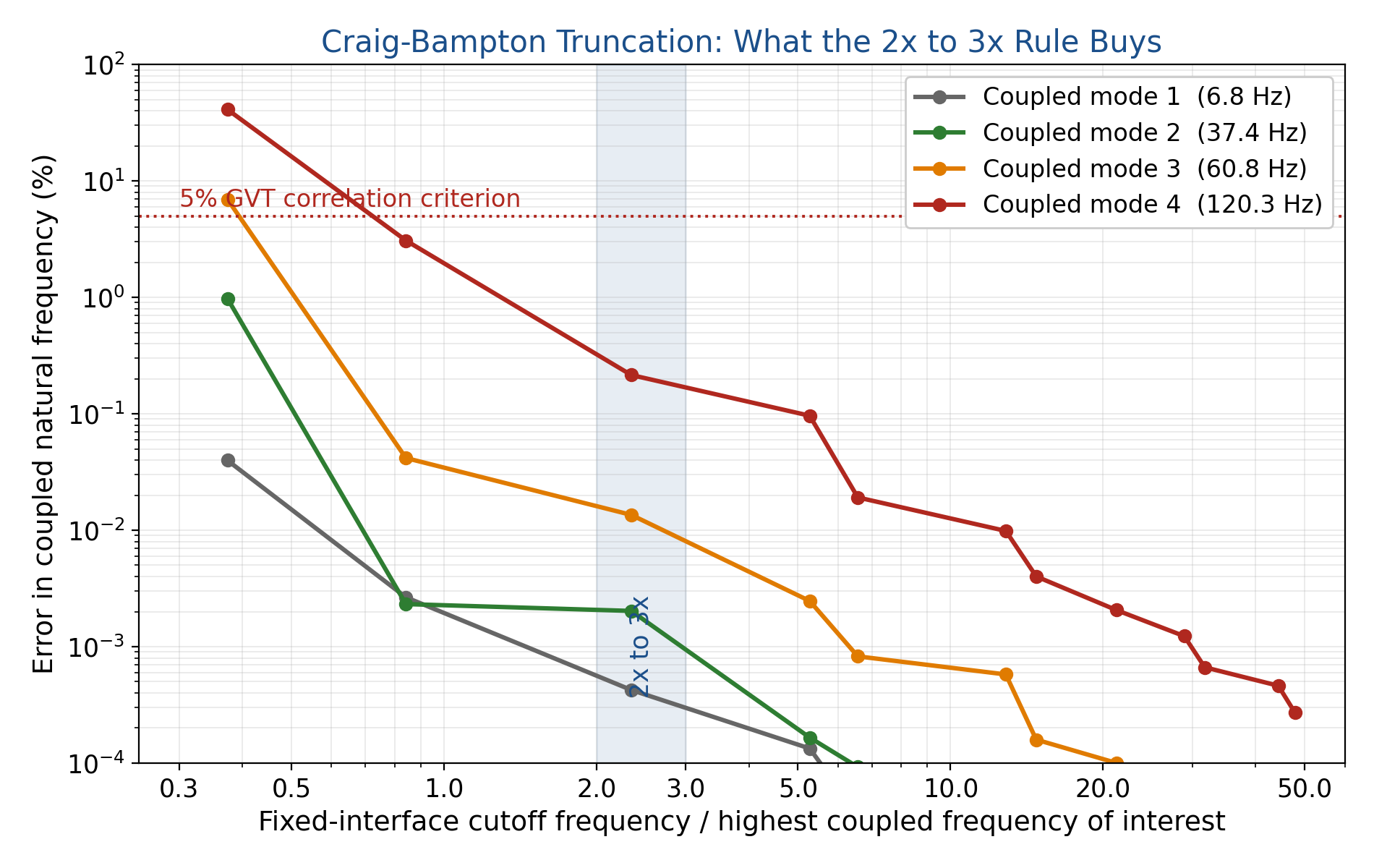
Three things are visible in Figure 4. First, the rule of thumb is well calibrated: at a cutoff ratio of 2.34 the worst frequency error across the band is 0.22 percent, an order of magnitude inside the five percent criterion normally applied to ground vibration test correlation. Second, the fundamental mode is essentially converged from the first retained mode onward — 0.04 percent with a single fixed-interface mode — which is the constraint modes doing their work. Third, the penalty for truncating too early is not gentle. Cutting off below the top of the band puts 41 percent error into the highest coupled mode, and a model in that condition will not be caught by looking at the first mode or by any check on total mass.
Coupled Loads Analysis With a Craig-Bampton Model
The launch vehicle and spacecraft community settled this argument decades ago, for exactly the reason above: when payload and vehicle have comparable interface impedance, neither one’s environment can be specified independently of the other. A heavy store on a pylon is the same problem with different nouns. The vendor delivers a Craig-Bampton reduction of the pylon and store; the airframer assembles it with the wing model and runs the coupled analysis.
What that fixes is structural rather than incremental. The impedance coupling is automatic, so notching falls out of the physics instead of being applied as a correction factor. The coupled modes are correct, including store pitch and yaw modes interacting with wing bending and torsion — which the airframer needs anyway for flutter clearance. Interface forces are recovered directly. Most importantly, the airframer applies the actual unsteady pressure field from CFD or the wind tunnel to the coupled system, which is the only place that forcing physically exists, and the result is a set of time-consistent, phase-correct stresses at all locations at once. Multiaxial rainflow becomes legitimate, and superposition with the quasi-static maneuver loads happens naturally in the time domain rather than by combining spectra after the fact.
Mechanically, the delivery is the reduction described above — boundary degrees of freedom at the physical attach points, fixed-interface modes carried to two or three times the highest frequency of interest — together with output transformation matrices for stress and internal load recovery at the fracture critical locations. The airframer runs the assembly and returns recovered quantities through the vendor’s transformation matrices. That also resolves the proprietary data problem in both directions, since neither party has to release detailed geometry.
| Verification the airframer should require, and the vendor should run first | Criterion |
|---|---|
| Rigid body mass check, $T^{T} M T$ | matches measured mass, CG, and inertia tensor |
| Free-free modes of the reduced model | match the full model over the band of interest |
| Strain energy under rigid body motion | essentially zero |
| Residual flexibility or attachment modes | included, or truncation convergence demonstrated |
| Correlation to a ground vibration test of the store on the pylon | frequency within about 5%, cross-orthogonality 0.9 or better on the modes that matter |
This Is Already Done on Aircraft
A reasonable objection at this point is that all of the above is spacecraft practice being imported into a world that does not work that way. It is not. The reduced-model exchange is established aircraft practice in at least three places, and the closest precedent is not the launch vehicle at all — it is the engine.
Engines. Boeing has described the Craig-Bampton method as central to its aeroelastic process for flight loads and flutter analysis, and as extensively applied in propulsion dynamics for windmilling, fan blade out loads, and engine vibration related noise. For the vibro-acoustic case the airframe and the acoustic fluid model are reduced down to the interface with the engine, and — this is the part that matters here — that superelement package is delivered to the engine manufacturers as boundary matrices and output transformation matrices, which lets the engine companies evaluate how different bearing and mount designs affect interior cabin noise while the airframer’s proprietary content stays inside the reduction. That is the exact arrangement being proposed for stores, running in the opposite direction, between an airframer and a component vendor, on production programs. It is worth noting in passing that the same source records that the seminal 1968 paper was written by Roy Craig of the University of Texas and Mervyn Bampton, who was a Boeing structures engineer — the method did not arrive from outside the airframe community, it started there.
Store flutter clearance. Coupled aircraft-plus-store models are not exotic; they are how store flutter clearance is done. Published work routinely builds a full-aircraft finite element model including pylons and external stores, couples it to a doublet-lattice aerodynamic model, and validates the assembly against ground vibration test data across several store configurations. The NATO educational material on flutter clearance with external stores describes the same practice in component terms, with secondary modes representing substructures such as an external store and attachment modes introduced to vary the connection stiffness between the store and the wing. If an airframer is clearing a store for flutter, a correlated coupled model of that store on that wing already exists.
Store configuration studies. Component mode synthesis was adapted to this exact problem nearly forty years ago. Karpel’s fictitious mass method was published in the Journal of Aircraft in 1988 under the title “Efficient Vibration Mode Analysis of Aircraft With Multiple External Store Configurations,” and the modal coupling techniques that grew out of it were developed specifically so that many store configurations on a fighter could be evaluated without recomputing the whole aircraft each time. The configuration-count objection raised below is a real difficulty, but it is not an unsolved one.
What is missing, then, is not the method, the software, the standards, or the industrial experience. All of that is in place. What is missing is the application of the method to the store vibration environment and the fatigue and fracture chain that hangs off it. That path still runs on specified spectra, and it is the one place in the store certification process where the impedance problem is neither solved nor acknowledged.
The Coupled Model Usually Already Exists
This changes the shape of the request considerably, and it is the practical point on which the whole argument turns. Standing up a coupled loads process for store vibration environments — model deliveries, iteration cycles, released recovered loads, schedule and data rights — is a program, and program offices are right to be wary of it. But on most aircraft carrying heavy stores, the coupled aircraft-and-store model was already built for flutter clearance, already correlated to a ground vibration test, and is already maintained by the aeroelasticity group.
So the ask is not “build a coupled loads capability.” It is “let the loads and fatigue group use the model the flutter group already built and validated.” Recovering interface forces and stresses from an existing correlated model is a far easier proposition than creating a new process, and it has the additional merit that the two disciplines then stop working from different structural representations of the same hardware — which, when it happens, is a defect in its own right.
Where It Is Harder Than It Sounds
Store attachments are among the worst nonlinearities in the airframe. Preloaded sway braces, lug and hook clearance, friction, bumpers, and ejector feet all produce amplitude-dependent stiffness, and measured frequencies shift with sway brace torque and with fuel state. Craig-Bampton is linear. The practical answer is to bound the behavior by delivering several reduced models at high and low preload and at the relevant mass states, and letting the coupled analysis run the matrix — which then collides with the second difficulty, configuration count. Symmetric and asymmetric loadings, adjacent stores, and fuel states multiply quickly, and a rational down-select is required rather than an exhaustive sweep. The flutter community’s modal coupling methods noted above exist precisely because this combinatorial problem had to be solved once already, and they are worth borrowing rather than reinventing.
Damping is a recurring trap, since the coupled system’s modal damping is not inherited from either component and the wing’s aerodynamic damping is often far higher than the 3% critical or $Q = 10$ that a vendor would assume in isolation. Interface modeling is another: an RBE2 spider at the attach points reintroduces local stiffening and quietly recreates the rigid interface the coupled analysis was meant to escape. Model the fittings, or use RBE3. Finally, the binding constraint is usually contractual rather than technical. “Here is your PSD” is a deliverable. A coupled loads cycle with iteration and released recovered loads is a program, with schedule and data rights attached.
Middle Ground
If a full coupled loads analysis cannot be obtained, the following are worth pursuing in roughly this order.
- Ask whether a flutter model already exists for this store on this wing, and whether it has been correlated to a ground vibration test. If the answer is yes, most of the technical work is already paid for and the discussion is about access rather than about analysis.
- Ask for the interface apparent mass or accelerance matrix at the attach points along with the PSD. The vendor can then perform the coupling itself in the frequency domain, which is coupled loads analysis with the roles reversed, or at minimum compute a defensible notch.
- Ask for a dual specification — an interface force PSD or force limit spectrum alongside the acceleration PSD. This is routine in spacecraft vibration testing and it caps the over-prediction directly.
- Apply semi-empirical force limiting with $C^2$ between 2 and 5. Crude, and it requires a mass ratio estimate, but as shown above it recovers most of the error for very little effort.
- Ask for a reduced model of the wing instead of delivering one of the store. This is sometimes easier to negotiate, and the coupling mathematics is identical.
- Plan on a strain survey. Store fatigue and fracture certification generally ends up leaning on instrumented flight test regardless, which argues for treating the base drive analysis as a sizing tool and reserving the fracture assessment for a load spectrum that contains real impedance and real mean stress.
References
T. Scharton, Force Limited Vibration Testing Monograph, NASA RP-1403, 1997.
R. Craig and M. Bampton, “Coupling of Substructures for Dynamic Analyses,” AIAA Journal, Vol. 6, No. 7, 1968.
J. F. Castro, “An Historical Perspective on Boeing’s Influence on Dynamic Structural Analysis Numerical Simulation,” Boeing Technical Journal, summarized in Innovation Quarterly, Vol. 1, Issue 4, May 2017, pp. 28-31.
M. Karpel, “Efficient Vibration Mode Analysis of Aircraft With Multiple External Store Configurations,” Journal of Aircraft, Vol. 25, No. 8, 1988, pp. 747-751.
NATO STO-EN-SCI-277, Flutter Clearance of Aircraft with External Stores, 2018.
NASA-STD-7001, Payload Vibroacoustic Test Criteria.
MIL-STD-8591, Airborne Stores, Suspension Equipment and Aircraft-Store Interface, 12 December 2005.
Related free ebooks are available at Tom’s Ebooks.