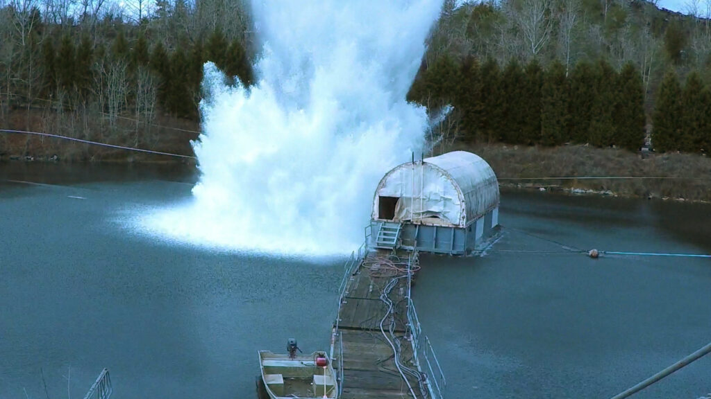
The image shows a MIL-S-901D Barge Test. A reader recently wrote in with two requests: (1) blog posts on surface ship shock and shock response spectra derived from acceleration data, and (2) coverage of underwater explosion (UNDEX) shock effects on submerged components such as batteries. This post is a response to both, tying together the UNDEX environment, shock response spectra, the Dynamic Design Analysis Method (DDAM), modal combination methods, MIL-DTL-901 qualification testing, and the stress–velocity relationship. Thank you to the reader for the excellent suggestion.
1. The UNDEX Threat Environment
A naval vessel subjected to a nearby underwater explosion experiences a sequence of loading events, each with its own frequency content and damage potential:
The primary shock wave. Detonation of the charge produces a steep-fronted pressure wave that propagates through the water at approximately the acoustic speed (~1500 m/s, ~5000 ft/s). At a fixed field point, the pressure history is well approximated by an exponential decay:
\[ P(t) = P_{max}\, e^{-t/\theta} \]
Cole’s classic similitude equations for TNT give the peak pressure and decay constant as functions of charge weight \(W\) (lbf) and standoff distance \(R\) (ft):
\[ P_{max} \approx 21{,}600 \left( \frac{W^{1/3}}{R} \right)^{1.13} \;\; \text{psi} \]
\[ \theta \approx 0.058\, W^{1/3} \left( \frac{W^{1/3}}{R} \right)^{-0.22} \;\; \text{ms} \]
The decay constant is typically a fraction of a millisecond to a few milliseconds. The shock wave is thus a broadband, high-frequency input. It drives hull plating, wetted appendages, and hull-mounted equipment directly.
The gas bubble pulse. The detonation products form a gas bubble that expands past equilibrium, collapses, and re-expands, radiating a secondary pressure pulse on each collapse. The first bubble period for TNT is given by the Willis equation:
\[ T_1 \approx \frac{4.36\, W^{1/3}}{(D + 33)^{5/6}} \;\; \text{s} \]
where \(D\) is the charge depth in feet. The bubble pulse peak pressure is only on the order of 10–20% of the shock wave peak, but its energy is concentrated at low frequency — often near the first vertical bending modes of the ship girder. This is the mechanism behind hull whipping, which can break a ship’s back even when the shock wave itself does not rupture plating. Bubble migration toward the free surface (or toward the hull) complicates the geometry.
Bulk cavitation and reloading. The shock wave reflects from the free surface as a rarefaction. Since water cannot sustain significant tension, a region of bulk cavitation forms below the surface. Its subsequent closure produces a reloading pulse. Near the hull, local cavitation at the fluid–structure interface similarly cuts off and then reloads the plating.
2. Shock Factor
Navy practice condenses the attack geometry into a single severity parameter, the shock factor. In its simplest form:
\[ SF = \frac{\sqrt{W}}{R} \]
with \(W\) in pounds of TNT-equivalent and \(R\) in feet. Variants weight the result by the incidence angle of the shock wave on the hull or keel, e.g. a keel shock factor of the form
\[ KSF = \frac{\sqrt{W}}{R}\left( \frac{1 + \sin\phi}{2} \right) \]
where \(\phi\) describes the elevation angle of the charge relative to the keel. The shock factor is proportional to the free-field energy flux density reaching the hull and correlates reasonably well with the initial vertical “kickoff” velocity imparted to the ship structure. Design and test severities are specified in terms of shock factor, with the specific values being classified or distribution-restricted.
3. What the Ship Structure Does with the Input
The shock wave arrives at the hull as a pressure transient measured in thousands of psi lasting a millisecond or so. The structural response, however, is filtered by the ship itself:
Hull plating and hull-mounted foundations see high-acceleration, high-frequency motion. Innerbottom and lower deck structure responds with somewhat lower acceleration but substantial velocity change. Upper decks and mast structures act as multi-stage mechanical filters — the high-frequency content is attenuated, but deck flexural modes in the tens of Hz can amplify the mid-band motion delivered to mounted equipment.
A useful mental model, going back to the pioneering measurements that underpin DDAM, is that ship shock motion at an equipment foundation is displacement-limited at low frequency, velocity-limited at mid frequency, and acceleration-limited at high frequency. On a tripartite pseudo-velocity plot, the design environment looks like a trapezoid. This is precisely why pseudo-velocity shock response spectra are the natural currency of naval shock work — more on that shortly.
4. Shock Response Spectra from Measured Acceleration Data
The reader asked specifically about deriving shock response spectra (SRS) from acceleration data. The SRS answers the question: if a family of single-degree-of-freedom (SDOF) oscillators, each with a different natural frequency but common damping, were mounted on the measured motion, what peak response would each experience?
The recipe for ship shock data is the same as for pyrotechnic or seismic data, with a few conventions:
Each SDOF system is defined by natural frequency \(f_n\) and amplification factor \(Q\), where \(Q = 1/(2\zeta)\). The standard is \(Q = 10\) (5% damping). The natural frequency array is typically spaced at 1/6 or 1/12 octave increments; for ship shock, a range of roughly 1 to 1000 Hz captures both girder whipping and equipment-level response. The absolute acceleration response of each oscillator is computed with the Smallwood ramp-invariant digital recursive filtering relationship, which is the de facto industry algorithm and is exact for a piecewise-linear (ramp-invariant) representation of the input. Both positive and negative spectra should be computed and plotted, since asymmetry between them can flag zero-shift, clipping, or other measurement pathologies. The sample rate should be at least ten times the highest natural frequency of interest for accurate peak capture with the standard algorithm.
The pseudo-velocity SRS is then formed from the relative displacement response \(Z\):
\[ PV(f_n) = \omega_n \, Z_{max}(f_n), \qquad \omega_n = 2\pi f_n \]
and plotted on tripartite (four-coordinate) log-log paper, where constant-displacement and constant-acceleration lines appear as diagonals. Ship shock spectra plotted this way display the characteristic velocity-limited plateau in the mid band. My free SRS tutorial papers and the Vibrationdata MATLAB GUI package both include SRS and PV-SRS tools that implement the Smallwood algorithm, and I have posted several worked examples on this blog using field data — most recently accelerometer measurements from monuments and infrastructure during my travels.
One caution particular to UNDEX data: measured hull accelerations can contain very high-frequency, high-g content from plating response and cavitation closure that is real but structurally benign for internal equipment. Velocity-based interpretation, and integration checks on the acceleration record (net velocity change, displacement drift), are essential quality-control steps before an SRS is accepted as an equipment design basis.
5. The Stress–Velocity Connection
Why the emphasis on pseudo-velocity? Because modal velocity maps directly to dynamic stress. For a traveling wave in a rod, or equivalently for the modal response of simple structures, the peak stress is:
\[ \sigma_{max} = k\, \rho\, c \, v_{max} \]
where \(\rho\) is mass density, \(c = \sqrt{E/\rho}\) is the longitudinal wave speed, \(v_{max}\) is the peak modal velocity, and \(k\) is a constant of order unity that depends on geometry and boundary conditions (\(k=1\) for the rod; values up to about \(\sqrt{3}\) or somewhat higher arise for beams and plates). This is the relationship I formalized in my “Rev Q” stress–velocity paper, building on the work of Hunt, Gaberson, and Chalmers.
For steel, \(\rho c \approx 146\) psi per in/s. Gaberson’s famous severity threshold of 100 in/s of pseudo-velocity thus corresponds to roughly 14.6 ksi of modal stress in a steel rod-like member — a meaningful fraction of yield for ordinary structural steels once stress concentration and \(k\) factors are applied. Naval shock environments routinely exceed 100 in/s in the velocity-controlled band, which is exactly why ship equipment, foundations, and mounts require deliberate shock design rather than reliance on static margins.
The stress–velocity relationship also explains why DDAM design values, discussed next, are expressed in terms of a limiting velocity as well as a limiting acceleration.
6. DDAM — The Dynamic Design Analysis Method
DDAM is the U.S. Navy’s standard analytical method for qualifying shipboard equipment and foundations against UNDEX shock. It originated with Belsheim and O’Hara at the Naval Research Laboratory (NRL Memorandum Report 1396, 1963) and is implemented today per NAVSEA 0908-LP-000-3010 and related design data sheets. Conceptually, DDAM is a response-spectrum modal analysis — a first cousin of seismic response spectrum analysis — but with two distinctive naval features: modal-weight-dependent design values and the NRL modal combination rule.
6.1 Why the design values depend on modal weight
Shipboard shock measurements revealed an interaction effect sometimes called the “shock spectrum dip”: heavy equipment dynamically loads its foundation and the surrounding ship structure, reducing the motion delivered at the mounting interface. A 200-lb electronics cabinet and a 40,000-lb reduction gear on the same deck do not see the same effective spectrum. DDAM captures this by making the design values decreasing functions of the modal effective weight.
6.2 The procedure
Step 1 — Modal analysis. Build a model of the equipment plus its foundation, fixed at the ship attachment interface, and extract natural frequencies \(\omega_a\) and mode shapes \(\phi_{ia}\).
Step 2 — Participation factors and modal weights. For each mode \(a\) and shock direction, compute the participation factor
\[ \Gamma_a = \frac{\sum_i w_i \, \phi_{ia}}{\sum_i w_i \, \phi_{ia}^2} \]
and the modal effective weight
\[ \bar{W}_a = \frac{\left( \sum_i w_i \, \phi_{ia} \right)^2}{\sum_i w_i \, \phi_{ia}^2} \]
where \(w_i\) are the lumped weights. The modal weights sum to the total weight; Navy practice is to retain enough modes to capture at least 80% of the total in each shock direction.
Step 3 — Shock design values. For each mode, the design acceleration \(A_a\) (in g) and design velocity \(V_a\) (in/s) are computed from coefficient equations that depend on ship type (surface ship vs. submarine), mounting location (hull, deck, or shell plating), shock direction (vertical, athwartship, fore-aft), and design philosophy (elastic vs. elastic-plastic). The governing modal design value is the lesser of the acceleration- and velocity-based values, with a floor:
\[ D_a = \max\!\left[ \min\!\left( A_a, \; \frac{\omega_a V_a}{g} \right), \; 6\ \text{g} \right] \]
This is the trapezoidal spectrum in equation form: low-frequency modes are velocity-controlled, high-frequency modes are acceleration-controlled.
The official coefficients reside in NAVSEA 0908-LP-000-3010 and are distribution-restricted, but the original unclassified interim values from NRL 1396 are widely reproduced in the open literature (e.g., Scavuzzo and Pusey) for illustration. For a surface ship, hull-mounted equipment, elastic design, vertical direction, with \(\bar{W}_a\) in kips:
\[ A_a = 20 \, \frac{(37.5 + \bar{W}_a)(12 + \bar{W}_a)}{(6 + \bar{W}_a)^2} \;\; \text{g} \]
\[ V_a = 60 \, \frac{(12 + \bar{W}_a)}{(6 + \bar{W}_a)} \;\; \text{in/s} \]
Athwartship and fore-aft directions use fractional multipliers of the vertical values. Note how both expressions decrease as modal weight grows — the spectrum dip in action.
A quick numerical illustration. Take \(\bar{W}_a = 2\) kips. Then \(A_a = 20(39.5)(14)/(8)^2 \approx 173\) g and \(V_a = 60(14)/(8) = 105\) in/s. The crossover frequency between the velocity- and acceleration-controlled regimes is
\[ f_c = \frac{A_a \, g}{2\pi V_a} = \frac{(173)(386)}{2\pi (105)} \approx 101 \;\text{Hz} \]
So for this modal weight, modes below about 100 Hz are designed to \( \omega_a V_a \) and modes above it to 173 g, with 6 g as the minimum in all cases. Note also that 105 in/s is comfortably above Gaberson’s 100 in/s severity threshold — the velocity design value alone tells you this is a serious stress environment.
Step 4 — Modal forces and stresses. Apply the equivalent static force set for each mode,
\[ F_{ia} = w_i \, \phi_{ia} \, \Gamma_a \, D_a \]
solve for member loads and stresses mode by mode, then combine.
7. Modal Combination Methods
Since modal peaks do not occur simultaneously, some statistical combination rule is required. Several are in common use across the shock and seismic worlds:
Absolute sum (ABSSUM). Adds the magnitudes of all modal responses. Guaranteed conservative, usually excessively so, since it assumes all modal peaks coincide in time and sign.
Square root of the sum of the squares (SRSS). The workhorse of seismic analysis for well-separated modes. It can, however, underpredict when one mode dominates or when modes are closely spaced.
Complete quadratic combination (CQC). The seismic community’s refinement of SRSS, adding cross-correlation terms between closely spaced modes. Appropriate for earthquake response spectrum analysis per ASCE 7 and similar codes.
The NRL sum. DDAM mandates its own rule: take the largest single modal response in absolute value, and add it to the SRSS of all remaining modes:
\[ R = |R_b| + \sqrt{ \sum_{a \neq b} R_a^2 } \]
where mode \(b\) is the mode producing the largest response of the quantity of interest (evaluated stress point by stress point, not globally). The NRL sum sits between SRSS and the absolute sum in conservatism. Its rationale is that in shock response one mode frequently dominates, and SRSS alone would dilute its contribution; the NRL sum guarantees the dominant modal peak appears at full value while treating the remainder statistically. The computed NRL-sum stresses are then compared against allowables — yield-based for elastic design, with higher permissible values under the elastic-plastic option for ductile structures.
8. MIL-S-901 / MIL-DTL-901E Shock Testing
Analysis and test are complementary qualification paths. The venerable MIL-S-901D has been superseded by MIL-DTL-901E (2017), but the architecture is familiar:
Grades. Grade A items are essential to the safety and continued combat capability of the ship and must remain operational through the shock event. Grade B items need only avoid becoming a hazard to personnel or to Grade A items — they may fail, but they may not become shrapnel, fire sources, or flooding paths.
Classes. Class I equipment is qualified without resilient mounts (hard-mounted); Class II is qualified with its resilient mounts installed; Class III covers both configurations.
Test machines. The Lightweight Shock Machine (LWSM) is a swinging-hammer anvil-plate machine for items up to roughly 550 lb, delivering a series of hammer blows from increasing drop heights in multiple orientations. The Medium Weight Shock Machine (MWSM) uses a 3000-lb hammer striking an anvil table for equipment up to several thousand pounds. Heavyweight items go to sea: they are mounted on a Floating Shock Platform (FSP) or Large Floating Shock Platform, and a series of explosive charges is detonated at progressively decreasing standoff distances, culminating in a severe design-level shot. The FSP series is the closest available approximation to the real UNDEX environment, complete with water-borne loading, fluid–structure interaction, and realistic foundation impedance.
Test versus DDAM. Items too large, too heavy, or too dangerous to test — main propulsion machinery, large switchboards, complete mast assemblies — are qualified by DDAM or by transient shock analysis with Navy-approved inputs, sometimes anchored by extension from tested similar items. Measured FSP acceleration data, reduced to shock response spectra exactly as described in Section 4, is a principal source for validating both the analytical models and the design value framework.
9. UNDEX Effects on Submerged and Internal Components — Batteries
The reader’s second request concerned submerged components such as batteries. Several distinct physics threads come together here.
9.1 Fluid–structure interaction
For wetted structure — shell plating, appendages, free-flooded equipment — the water is a participant, not a bystander. Taylor’s flat-plate theory shows that a light, air-backed plate struck by a plane shock wave can acquire a kickoff velocity approaching twice the free-field fluid particle velocity before cavitation cuts off the loading, with the attained velocity governed by the ratio of the decay constant to the plate’s areal-mass time scale. Added (entrained) mass lowers the natural frequencies of wetted structure substantially relative to in-air values — a critical modeling consideration for sonar domes, rudders, and shell-mounted items. Modern practice couples finite element structural models to fluid volumes or to boundary-element / Doubly Asymptotic Approximation formulations for this class of problem.
9.2 The battery problem
Batteries are a uniquely demanding shock-qualification case because they combine large mass, brittle or fragile internal construction, stored chemical energy, and safety-critical function. They are typically Grade A, Class I, and heavyweight-test candidates.
Legacy lead-acid batteries (the classic submarine main storage battery) exhibit well-documented shock failure modes: cracking of cast plates and grids, shedding of active material paste (with attendant capacity loss and internal short risk), intercell connector and busbar fractures, terminal post failures, container and cover cracking, and electrolyte spill — the last being both a corrosion and a chlorine-gas hazard in a seawater environment. The large cell mass means modal effective weights are high, which moderates the DDAM design values, but the internal components are stress-raisers all the way down.
Lithium-ion systems, now entering naval service for unmanned vehicles, submarines, and shipboard energy storage, raise the stakes. Mechanical abuse of a lithium-ion cell — electrode buckling, current-collector tearing, separator puncture or crush — can create an internal short circuit, and an internal short can initiate thermal runaway with cell venting, fire, and cascade propagation through a module. The qualification problem is therefore not merely “does it still deliver current after the shot” but “is a latent internal short being seeded that manifests hours later.” Navy lithium battery safety certification (the NAVSEA S9310 process) accordingly layers abuse testing, fault propagation analysis, and system-level protections on top of the MIL-DTL-901E mechanical qualification.
Design mitigations follow directly from the physics discussed above:
Cell restraint and preload so that electrode stacks cannot displace relative to the case under the velocity-dominated mid-band input; potting or structural foam where thermal management permits; module and rack designs that keep the first internal resonances above the velocity-controlled band where feasible, pushing response into the acceleration-limited (and displacement-small) regime; resilient mounting (Class II) to attenuate high-frequency content — with careful attention to sway space, snubbing, and the large low-frequency displacements that soft mounts permit under a velocity-type shock; robust busbar and interconnect flexures so that relative motion between cells does not fatigue or fracture conductors; and battery management system electronics qualified to the same environment, since a BMS that resets or fails during the event defeats the protection scheme.
The stress–velocity relationship earns its keep here as a screening tool: given a pseudo-velocity SRS at the battery foundation, \(\sigma \approx k \rho c\, v\) provides an immediate first-order estimate of modal stress in busbars, brackets, and cell case walls before any finite element model exists.
10. Closing Thoughts
Surface ship shock design is a beautiful example of a complete engineering chain: explosion physics (Cole similitude), fluid–structure interaction (Taylor plates, cavitation), measured-data reduction (SRS via the Smallwood algorithm, pseudo-velocity tripartite plots), design abstraction (DDAM modal weights and design values), response statistics (the NRL sum), material limits (stress–velocity and Gaberson’s threshold), and validation by test (MIL-DTL-901E, culminating in the Floating Shock Platform). Each link informs the others, and each is worth a deeper post of its own — reader requests for any particular link are welcome.
I cover shock response spectra, pseudo-velocity, stress–velocity methods, and related shock analysis topics in depth in my upcoming continuing education course series beginning in September 2026, with IACET-accredited CEUs available. Details are at vibrationdata.com.
References
R.H. Cole, Underwater Explosions, Princeton University Press, 1948.
R.O. Belsheim and G.J. O’Hara, “Shock Design of Shipboard Equipment — Dynamic Design-Analysis Method,” NRL Memorandum Report 1396, U.S. Naval Research Laboratory, 1963.
NAVSEA 0908-LP-000-3010, Rev. 1, “Shock Design Criteria for Surface Ships,” Naval Sea Systems Command.
MIL-DTL-901E, “Shock Tests, H.I. (High-Impact) Shipboard Machinery, Equipment, and Systems, Requirements for,” 2017.
R.J. Scavuzzo and H.C. Pusey, Naval Shock Analysis and Design, SVM-17, Shock and Vibration Information Analysis Center.
G.I. Taylor, “The Pressure and Impulse of Submarine Explosion Waves on Plates,” 1941 (reprinted in Underwater Explosion Research, Vol. 1, ONR, 1950).
H.A. Gaberson, “Shock Severity Estimation,” Sound & Vibration, January 2012.
D.O. Smallwood, “An Improved Recursive Formula for Calculating Shock Response Spectra,” Shock and Vibration Bulletin, No. 51, 1981.
T. Irvine, “Shock and Vibration Stress as a Function of Velocity,” Rev Q, Vibrationdata, available at vibrationdata.com.
📌 Looking for a comprehensive guide on shock analysis and testing? Explore our Pyrotechnic Shock Resource Hub for an annotated directory of tutorials, standards, SRS synthesis methods, and aerospace case studies.
📌 Related Earthquake Engineering Knowledge Hub
This article is featured in our main Earthquake Engineering & Structural Dynamics Hub . Visit the hub to explore related articles on shock response spectra, time history analysis, seismic equipment qualification, and structural case studies.
1 thought on “Surface Ship Shock, SRS, DDAM, MIL-DTL-901, UNDEX”