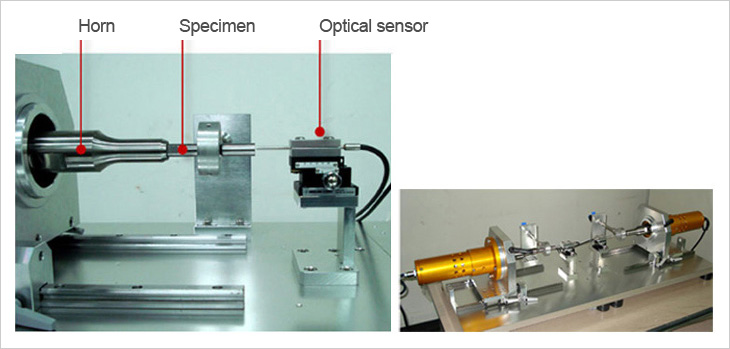
Ultrasonic Fatigue Tests - Vibrationdata Blog

Image Courtesy of http://www.mbrosia.co.kr/en/product/product0101.php

Ultrasonic fatigue testing at 20 kHz has become the standard method for characterizing material fatigue in the Very High Cycle Fatigue (VHCF) regime — beyond 10⁷ cycles, extending to 10⁹ (gigacycle) and beyond. At 20 kHz, a test that would require 11.6 days at 100 Hz completes in 14 minutes. This post covers the operating principle, specimen design, stress measurement and calculation methods — including the stress-velocity relationship — the burst-pause (pulse-pause) loading protocol for thermal management, and the engineering interpretation of VHCF results.

1. Motivation — The Very High Cycle Fatigue Regime

Classical fatigue testing at servo-hydraulic frequencies of 1–100 Hz reaches 10⁷ cycles in hours to days — sufficient for the traditional fatigue limit concept applicable to steels. But many engineering components accumulate far more cycles in service:

Application	Operating Frequency	Lifetime Cycles
Aircraft turbine blade	~200–400 Hz (1E)	10⁹ – 10¹⁰
Automotive engine component	~50–100 Hz	10⁸ – 10⁹
Railway axle	~3–10 Hz	10⁹ – 10¹⁰
Wind turbine drivetrain	~1–10 Hz	10⁸ – 10⁹
Power generation turbine	50–60 Hz	10¹¹

Conventional testing cannot reach these cycle counts in reasonable laboratory time. At 100 Hz, 10⁹ cycles requires 115 days of continuous testing per specimen. At 20 kHz, the same 10⁹ cycles completes in under 14 hours.

The VHCF regime also reveals fatigue behavior not captured by 10⁷-cycle testing. Many materials — including aluminum alloys, titanium alloys, and high-strength steels — do not exhibit a true endurance limit. The S-N curve continues to slope downward beyond 10⁷ cycles, and failures have been documented at 10⁹–10¹⁰ cycles at stress amplitudes well below the conventional fatigue limit. Crack initiation mechanisms also change: surface initiation dominant at lower cycles transitions to subsurface initiation at inclusions or microstructural inhomogeneities at VHCF, producing the characteristic “fish-eye” fracture morphology.

2. Operating Principle

Ultrasonic fatigue testing is based on longitudinal resonance of the specimen assembly at 20 kHz. The complete mechanical chain consists of:

Piezoelectric transducer: Converts a 20 kHz electrical signal from the generator into mechanical vibration via the inverse piezoelectric effect. Typical peak-to-peak displacement at the transducer output: 10–20 μm.
Booster (amplitude transformer): A stepped horn that amplifies or attenuates the displacement amplitude by a fixed geometric ratio (typically 1:1 to 1:3).
Acoustic horn (sonotrode): A second amplitude transformer, further amplifying displacement to the level required for the target stress amplitude in the specimen. Custom-designed for each specimen geometry and material.
Specimen: An hourglass-profile bar whose geometry is tuned so that its natural frequency of longitudinal vibration matches 20 kHz exactly.

The entire assembly — transducer, booster, horn, specimen — must resonate as a single system at 20 kHz. Each element is designed to be a half-wavelength (λ/2) resonator, so that displacement antinodes occur at the free ends and a displacement node (stress antinode) occurs at the midpoint. The specimen minimum section is placed at the displacement node — the location of maximum strain and maximum stress.

The wavelength of a longitudinal wave in the specimen material is:

λ = c / f = √(E/ρ) / f

For steel at 20 kHz: c = 5100 m/s, λ = 255 mm. A half-wave steel specimen is therefore ~127 mm long. For aluminum (c ≈ 5100 m/s as well): similar length. For titanium (c ≈ 4900 m/s): λ/2 ≈ 122 mm. The hourglass geometry is superimposed on this half-wave constraint to concentrate stress at the midpoint.

The standard loading mode is fully reversed tension-compression at stress ratio R = −1. Some configurations achieve bending modes for surface-sensitive fatigue studies or components where bending dominates in service.

3. Specimen Design

The specimen geometry must simultaneously satisfy two constraints:

Resonance frequency exactly at 20 kHz (the system operating frequency)
Maximum stress concentrated at the minimum cross-section (gauge section)

The standard hourglass specimen profile uses a smooth concave radius connecting the grip ends to the reduced gauge section. The profile is optimized by finite element analysis (FEA), iterating on the gauge diameter and radius until the first longitudinal mode falls at 20 kHz. Common gauge section diameters range from 3 to 6 mm for metallic specimens.

The design output is a stress-to-displacement calibration factor K:

σ_a = K × u₀

where σ_a is the stress amplitude at the gauge section (MPa) and u₀ is the displacement amplitude at the specimen end or horn tip (μm). K is computed from the FEA mode shape and has units of MPa/μm. Typical values range from 5–30 MPa/μm depending on material and specimen geometry.

The linear relationship between stress amplitude and displacement amplitude has been validated experimentally by strain gauges and laser Doppler vibrometry across a wide range of materials and stress levels, provided the specimen remains in the elastic regime — which is the case for VHCF testing where stress amplitudes are below yield strength.

4. Stress Measurement and Calculation

Because the test is displacement-controlled, stress at the gauge section is not measured directly by the machine. Three approaches are used:

4.1 Strain Gauges

A foil strain gauge bonded near the gauge section measures surface strain, from which stress is computed as:

σ = E ε

This is the most direct method. However, standard foil gauges have limited dynamic response and are unreliable at 20 kHz. Specialized PVDF film gauges or miniature semiconductor gauges can extend the usable frequency range. Additionally, specimen heating at higher stress amplitudes can compromise gauge adhesive and alter the calibration. Strain gauges are therefore used primarily for initial calibration at moderate stress levels, establishing the K factor, rather than for continuous monitoring throughout the test.

4.2 FEA Calibration with Displacement Measurement

The most common production approach:

Compute K = σ_max / u₀ from the FEA mode shape
Measure u₀ continuously during the test using a non-contact sensor (laser displacement sensor or eddy-current probe) at the specimen end or horn tip
Compute σ_a = K × u₀ in real time

The machine control loop maintains constant u₀ (and therefore constant σ_a) throughout the test. This is the standard approach per ASTM E2368 and ISO 1099.

4.3 Laser Doppler Vibrometry and the Stress-Velocity Relationship

A laser Doppler vibrometer (LDV) measures the instantaneous surface velocity v(t) at any accessible point on the specimen without contact. For a plane longitudinal wave propagating in a uniform bar, particle velocity and stress are related by the acoustic impedance of the material:

σ = ρ c v

where:

ρ = material density (kg/m³)
c = longitudinal wave speed = √(E/ρ) (m/s)
v = particle velocity (m/s)

This is the stress-velocity relationship published by Irvine (Stress and Strain as a Function of Velocity, Rev Q, VibrationData). At 20 kHz with displacement amplitude u₀, the peak particle velocity is:

v_peak = 2π f u₀

So the peak stress amplitude is:

σ_peak = ρ c × 2π f u₀

Numerical example — steel at 20 kHz:
ρ = 7800 kg/m³, c = 5100 m/s, f = 20,000 Hz, u₀ = 10 μm
v_peak = 2π × 20,000 × 10×10⁻⁶ = 1.257 m/s
σ_peak = 7800 × 5100 × 1.257 = 49.9 MPa

Numerical example — aluminum at 20 kHz:
ρ = 2700 kg/m³, c = 5100 m/s, f = 20,000 Hz, u₀ = 10 μm
v_peak = 1.257 m/s
σ_peak = 2700 × 5100 × 1.257 = 17.3 MPa

Numerical example — titanium Ti-6Al-4V at 20 kHz:
ρ = 4430 kg/m³, c = 4900 m/s, f = 20,000 Hz, u₀ = 10 μm
v_peak = 1.257 m/s
σ_peak = 4430 × 4900 × 1.257 = 27.3 MPa

The acoustic impedance Z = ρc thus serves as a direct conversion factor between measurable velocity and stress:

Material	ρ (kg/m³)	c (m/s)	Z = ρc (MPa·s/m)	σ/v (MPa per m/s)
Steel (4340)	7800	5100	39.8	39.8
Aluminum (6061)	2700	5100	13.8	13.8
Titanium (Ti-6Al-4V)	4430	4900	21.7	21.7
Magnesium (AZ31)	1770	5200	9.2	9.2
Inconel 718	8190	5490	44.9	44.9

Applications of the Stress-Velocity Relationship in Ultrasonic Fatigue

Non-contact stress estimation: LDV measurement of surface velocity at any accessible location, combined with the FEA mode shape, gives stress at the gauge section without bonded sensors.
Real-time monitoring: Velocity is continuously measurable during the test. A drop in acoustic impedance (v increasing for constant displacement) signals modulus reduction from fatigue damage accumulation — an early warning indicator prior to macroscopic fracture.
Independent cross-check on FEA calibration: The FEA-derived K factor can be verified by measuring v at the specimen end and computing σ = ρc·v, then comparing to the FEA prediction. Agreement within 5% is typical for well-designed specimens.
Scanning LDV for stress mapping: A scanning LDV measures the velocity field over the specimen surface, providing a distributed stress map without a strain gauge array — particularly useful for complex geometry specimens.

Limitation: The relation σ = ρcv applies strictly to plane wave propagation in a uniform bar. Near the hourglass notch root, the stress field is three-dimensional and the stress concentration factor K_t elevates the true peak stress above the plane-wave estimate. FEA correction for the notch geometry remains necessary for accurate gauge-section stress determination. The velocity measurement gives an excellent first-order result and a powerful experimental cross-check, but should be combined with FEA for precision work.

5. Specimen Self-Heating and Thermal Management

At 20 kHz, even small levels of material damping (hysteretic energy dissipation per cycle) generate significant heat because the cycle rate is 20,000 per second. The temperature rise in a specimen under continuous sinusoidal loading at 20 kHz can reach tens to hundreds of degrees Celsius within seconds, depending on the material damping and stress amplitude.

This is a fundamental problem because:

Elevated temperature alters fatigue behavior — most metals exhibit higher fatigue life at elevated temperature due to recovery mechanisms, making high-frequency test results non-representative of room-temperature service.
Temperature rise changes the elastic modulus, shifting the resonant frequency away from 20 kHz and altering the stress-to-displacement calibration factor K.
Thermal gradients introduce residual stresses that modify crack initiation behavior.
For titanium alloys, elevated temperature can activate dwell fatigue mechanisms not present at room temperature.

Materials with high damping — polymers, composites, some magnesium alloys — are particularly susceptible. Metals with low damping (steel, aluminum, titanium) heat more slowly but still require thermal management at higher stress amplitudes.

Thermal Management Methods

Forced air cooling: A focused air jet directed at the specimen gauge section. Effective for moderate stress amplitudes in metals. Compressed air or vortex tube cooled air (below ambient temperature) is used for higher heat generation rates.
Liquid cooling: For very high stress amplitudes or high-damping materials, the specimen gauge section is immersed in a cooling bath (water, oil, or liquid nitrogen for cryogenic testing). This also enables corrosion-fatigue testing by using the appropriate corrosive medium as the coolant.
Burst-pause (pulse-pause) loading: The most widely used method, described in detail in Section 6.
Infrared thermography monitoring: An IR camera monitors surface temperature continuously. The control system modifies the duty cycle or pauses the test when temperature exceeds a threshold (typically 5–10°C above ambient for metals).

6. Burst-Pause (Pulse-Pause) Loading Protocol

The burst-pause method applies the 20 kHz sinusoidal excitation in discrete bursts (pulses) separated by rest periods (pauses) during which the specimen cools passively or under forced air. This is the standard approach for metallic specimens in the VHCF regime.

Typical Parameters

Parameter	Typical Value	Notes
Pulse duration (t_on)	50–200 ms	At 20 kHz: 1000–4000 cycles per burst
Pause duration (t_off)	500–5000 ms	3–25× the pulse duration
Duty cycle	4–25%	t_on / (t_on + t_off)
Maximum temperature rise	< 5–10°C	Measured at gauge section surface
Effective test frequency	800–5000 Hz equivalent	Cycle rate = 20,000 × duty cycle

A common protocol for steel and titanium is t_on = 200 ms, t_off = 1800 ms (10% duty cycle), giving an effective cycle accumulation rate of 2000 cycles/second and maintaining specimen temperature within 5°C of ambient.

The number of fatigue cycles accumulated is counted from the pulse train:

N_total = f × t_on × n_bursts = 20,000 × t_on × n_bursts

The machine controller increments the cycle counter only during active pulses. The total elapsed real time is much longer than the accumulated fatigue time, but the fatigue damage corresponds only to the active loading cycles.

Temperature Evolution in Burst-Pause Loading

During each pulse, the specimen temperature rises approximately as:

ΔT_rise ≈ Q·t_on / (ρ c_p V)

where Q is the volumetric heat generation rate (proportional to damping coefficient and stress amplitude squared), c_p is the specific heat, and V is the active gauge volume. During the pause, the specimen cools exponentially toward ambient:

T(t) = T_ambient + ΔT_max × exp(−t / τ_cool)

where τ_cool is the thermal time constant of the specimen in its cooling environment. Pulse-pause parameters are chosen so that ΔT_max after each burst is small, and the specimen cools back to near-ambient before the next burst fires. Steady-state mean temperature (averaged over many cycles) stabilizes well below the thermal limit.

Effect of Pulse-Pause Parameters on Fatigue Results

For metals, fatigue life is generally insensitive to the burst-pause ratio provided the maximum temperature excursion is kept below ~10°C. Studies on steel and aluminum have shown that fatigue lives obtained with burst-pause loading at 20 kHz are consistent with conventional servo-hydraulic results when plotted on the same S-N curve, confirming that the burst-pause protocol does not introduce artificial frequency effects for these materials.

For polymers and composites, the pulse-pause parameters have a stronger influence on fatigue results, because these materials exhibit higher damping and stronger temperature-dependent fatigue behavior. Pulse-pause optimization for composites requires careful thermal characterization and is an active area of research.

Note: The burst-pause cycle count method must be used consistently when comparing results across laboratories. Some researchers report total elapsed time (which includes pause periods) rather than active fatigue cycles — an ambiguity that has led to apparent discrepancies in the literature. Cycle count should always mean cycles of mechanical loading at 20 kHz, not clock time.

7. Failure Detection

Specimen fracture at 20 kHz is detected by monitoring the resonant frequency of the assembly. As a fatigue crack propagates, it reduces the specimen stiffness and therefore lowers the resonant frequency. The machine control system detects a frequency drop below a threshold (typically 50–200 Hz from the nominal 20 kHz) and shuts down, recording the total cycle count at failure.

For VHCF testing, crack propagation occupies a very small fraction of total fatigue life. Studies on Inconel 718 have found that crack propagation from initiation to fracture consumes less than 1% of total fatigue life — the remaining 99%+ is crack initiation. This is in contrast to high-cycle fatigue at moderate cycle counts, where propagation can consume 20–50% of life.

Additional monitoring channels include:

Displacement amplitude (LDV or eddy current) — sudden increase signals stiffness loss
Acoustic emission — detects microcrack nucleation events prior to macroscopic frequency shift
Infrared thermography — localized hot spot at crack tip visible before frequency drop

8. VHCF Fracture Mechanisms

A key finding from ultrasonic fatigue testing is that the dominant crack initiation mechanism shifts with increasing cycle count:

Cycle Range	Dominant Initiation Site	Morphology
10⁴ – 10⁶	Surface slip bands, notches	Beach marks, radial lines from surface
10⁶ – 10⁷	Surface or near-surface defects	Transition zone
10⁷ – 10⁹	Subsurface inclusions, pores, grain clusters	“Fish-eye” fracture — circular crack front around internal defect
> 10⁹	Granular bright facet (GBF) around inclusion	Fish-eye with fine granular area (FGA) at inclusion

The fish-eye morphology is characteristic of VHCF. A subsurface inclusion (oxide, sulfide, carbide) or pore initiates a slow-growing crack in the absence of corrosive environment or stress concentration. The crack propagates radially outward under the applied stress field, producing a roughly circular fracture region visible on the fracture surface as a bright disc surrounded by the rougher fast-fracture zone. The inclusion is visible at the center of the fish-eye.

The Granular Bright Facet (GBF) is a fine-grained region immediately surrounding the inclusion, produced by repeated crack opening and closing over millions of cycles before the crack reaches a size sufficient for stable propagation. The GBF size is related to the threshold stress intensity factor ΔK_th of the material.

9. S-N Curve Behavior in the VHCF Regime

The S-N curve for many metals in the VHCF regime is not a horizontal asymptote (endurance limit) but a continuously declining or stepwise declining function:

Steels: Carbon and low-alloy steels exhibit a true endurance limit at ~10⁶–10⁷ cycles related to dislocation pinning by interstitial atoms. However, high-strength steels (hardness > 400 HV) show continued fatigue failure beyond 10⁷ cycles via subsurface inclusion initiation, with no true endurance limit.
Aluminum alloys: No true endurance limit; S-N curve continues to decline through 10⁹ cycles. VHCF failures in aluminum typically initiate at casting pores, constituent particles, or slip bands.
Titanium alloys: Ti-6Al-4V shows a “duplex” S-N curve — a change in slope around 10⁷ cycles corresponding to the transition from surface to subsurface initiation, but no horizontal asymptote.
Magnesium alloys: Similar to aluminum — no true endurance limit, with VHCF failures documented through 10⁹ cycles, particularly in corrosive environments.

The Basquin power law S-N relationship:

σ_a = σ’_f (2N_f)^b

applies in the finite life regime. In the VHCF regime, a dual-slope Basquin model is sometimes used to capture the slope change at the surface-to-subsurface transition:

For N < N_transition: σ_a = σ’_f1 (2N_f)^b₁
For N > N_transition: σ_a = σ’_f2 (2N_f)^b₂

where b₂ is typically shallower (less negative) than b₁, reflecting the slower crack propagation rate from subsurface initiation sites.

10. Frequency Effects and Test Validity

A critical question for ultrasonic fatigue testing is whether results at 20 kHz are representative of service behavior at 1–100 Hz. Frequency can affect fatigue through two mechanisms:

Strain rate sensitivity: Higher frequency means higher strain rate. For materials whose fatigue mechanisms are strain-rate sensitive (body-centered cubic steels with dynamic strain aging, some titanium alloys), results at 20 kHz may differ from those at low frequency.
Corrosion fatigue: Corrosive damage per cycle is time-dependent — at 20 kHz, the exposure time per cycle is 50 μs, compared to 10 ms at 100 Hz. In corrosive environments, ultrasonic fatigue substantially underestimates corrosion fatigue damage relative to low-frequency service. Corrosion fatigue testing must be conducted at representative frequencies.

For most structural metals (aluminum, steel, titanium) in benign environments, fatigue lives at 20 kHz agree well with servo-hydraulic results when plotted on the same S-N curve, validating the ultrasonic method for in-air VHCF characterization. Frequency effects are most significant for ferritic steels near the dynamic strain aging temperature range.

11. Summary

Parameter	Typical Value / Practice
Test frequency	20 kHz (15–22 kHz range across systems)
Cycle accumulation rate	20,000 cycles/second (continuous); 800–5000 cycles/second (burst-pause)
Time to 10⁹ cycles (continuous)	~14 hours
Stress ratio	R = −1 (standard); R = 0 or other ratios with mean load superposition
Stress measurement	FEA calibration + displacement sensor (primary); strain gauge (calibration); LDV + σ = ρcv (cross-check)
Thermal management	Burst-pause loading; forced air cooling; IR monitoring
Typical burst parameters (metals)	t_on = 200 ms, t_off = 1800 ms; ΔT < 5°C
Failure detection	Resonant frequency drop (> 50–200 Hz from 20 kHz)
VHCF crack initiation	Subsurface inclusions / fish-eye morphology beyond 10⁷ cycles
Governing standard	ASTM E2368; ISO 1099
Primary applications	Turbine blades, railway axles, automotive powertrain, aerospace structure

Ultrasonic fatigue testing at 20 kHz has transformed VHCF characterization from a multi-month laboratory undertaking into a routine test campaign. The combination of FEA-based stress calibration, laser Doppler vibrometry using the σ = ρcv stress-velocity relationship, burst-pause thermal management, and IR temperature monitoring provides a complete, validated test methodology for generating reliable S-N data through 10⁹–10¹⁰ cycles across the full range of structural metals.

References
Stanzl-Tschegg, S.E., Ultrasonic Fatigue, Fatigue and Fracture of Engineering Materials and Structures, Vol. 22, 1999, pp. 567–579.
Marines, I. et al., Ultrasonic fatigue tests on bearing steel AISI-SAE 52100 at frequency of 20 and 30 kHz, International Journal of Fatigue, Vol. 25, 2003, pp. 1037–1046.
Bathias, C., Paris, P.C., Gigacycle Fatigue in Mechanical Practice, Marcel Dekker, New York, 2005.
ASTM E2368, Standard Practice for Strain Controlled Thermomechanical Fatigue Testing.
ISO 1099, Metallic Materials — Fatigue Testing — Axial Force-Controlled Method.
Mayer, H., Fatigue crack growth and threshold measurements at very high frequencies, International Materials Reviews, Vol. 44, 1999, pp. 1–34.
Trujillo-Tadeo, J.J. et al., Microstructure and Corrosion Effects on ZW12 Fatigue Performance, IFC14, 2026.
Irvine, T., Stress and Strain as a Function of Velocity, Rev Q, VibrationData, 2024.
Irvine, T., ZW12 Magnesium Alloy: Microstructure, Corrosion, and Fatigue Performance, VibrationData Blog, 2026.